Pendulum Control
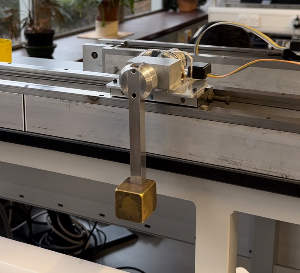
State space dynamic models and feedback control techniques applied to an inverted pendulum system, demonstrating pole placement, LQR control, and analysis of nonlinear effects.
Introduction
Purpose
State space dynamic models provide a powerful framework for modeling and analyzing complex real-world systems, enabling engineers to develop accurate and efficient control strategies. For example, state space models are widely used in the automotive industry to design advanced vehicle dynamics control systems, ensuring improved stability, handling, and safety. In the aerospace sector, state space models are employed to analyze and control aircraft dynamics, satellite attitude control systems, and missile guidance systems.
State feedback and pole placement techniques are essential tools for designing controllers that can modify the dynamics of real-world control systems to achieve desired performance characteristics. These techniques find extensive applications in robotics, where they are used to design controllers for manipulators, mobile robots, and humanoid robots, enabling precise motion control and trajectory tracking.
Objectives
- To derive and linearize equations of motion for crane and inverted pendulum arrangements of the system.
- To illustrate the use of state feedback and pole placement techniques to design a controller for the inverted pendulum system.
- To explain the limitations of pole placement control and effects of non-linearities in the system.
- To demonstrate the use of LQR control to design a controller for the inverted pendulum system.
Theory
Inverted Pendulum Dynamical System
 Figure 1: Inverted pendulum system
 Figure 2: Free body diagrams of the inverted pendulum system
The forces \(F_c\), \(F_f\) and \(R\) are the cable tension, friction force and vertical reaction acting on mass \(M\). The frictional force is defined below: \[F_f = F \text{sgn}(\dot{x}) \quad \text{where} \quad \text{sgn}(\dot{x}) = \begin{cases} 1 & \dot{x} > 0 \\ -1 & \dot{x} < 0 \\ \text{undefined for } \dot{x} = 0 \end{cases}\]
The vectors \(\mathbf{r}_P\) and \(\mathbf{r}_Q\) are the position vectors of masses \(M\) and \(m\) respectively: \[\mathbf{r}_P = x \mathbf{i} \quad \text{and} \quad \mathbf{r}_Q = (x-l\sin\theta) \mathbf{i} - l\cos\theta \mathbf{j}\]
These positions can be differentiated to find the momentum \(\mathbf{p}\) of the body: \[\mathbf{p} = \left[(M+m)\dot{x}-ml\dot{\theta}\cos\theta \right] \mathbf{i} + ml\dot{\theta}\sin\theta\mathbf{j}\]
The angular momentum about the point P is given by: \[\begin{align} \mathbf{h}_P &= \sum_i m_i(\mathbf{r}_i - \mathbf{r}_p) \times \mathbf{p}_i \\ &= m (\mathbf{r}_Q - \mathbf{r}_P) \times \dot{\mathbf{r}}_Q \\ &= \left[ -ml^2\dot{\theta} + ml\dot{x}\cos\theta \right] \mathbf{k} \end{align}\]
This can be differentiated and used with the equation below to find one of the equations of motion: \[\mathbf{Q}^{(e)} = \dot{\mathbf{h}}_P + \dot{\mathbf{r}}_P \times \mathbf{p}\]
Here the only external force that does not pass through P is the weight of the pendulum bob \(mg\) which is a distance \(l\sin\theta\) from P, and so the torque acts in the \(+\mathbf{k}\) direction. The equation of motion is then: \[mgl\sin\theta = ml\ddot{\theta} - ml\ddot{x}\cos\theta \tag{1}\]
From differentiating the linear momentum \(\mathbf{p}\) and from Newton’s second law: \[\dot{\mathbf{p}} = \left[F_c - F_f \right] \mathbf{i} + \left[ R - (m+M)g \right]\mathbf{j}\]
From considering the unrestrained \(\mathbf{i}\) direction the equation of motion is shown to be: \[(M+m)\ddot{x} - ml\ddot{\theta}\cos\theta + ml\dot{\theta}^2\sin\theta = F_c - F_f \tag{2}\]
However, the force in the cable \(F_c\) is required to be in terms of the torque \(T\) by the motor. This is found from considering the angular momentum about the motor’s axis. The angular acceleration of the pulley is \(\ddot{\alpha}\) and the radius of the pulley is \(a\): \[\begin{align} Q &= I\ddot{\alpha} \\ aF_c - T &= -I\frac{\ddot{x}}{a} \\ \implies F_c &= \frac{T}{a} - \frac{I}{a^2}\ddot{x} \end{align}\]
This can be then substituted into equation (2) and rearranged to give the equation of motion in terms of the torque \(T\). This is shown below along with a simplified form of equation (1): \[\begin{align} \left( 1 + \frac{M}{m} + \frac{I}{ma^2} \right) \ddot{x} &= \frac{T}{ma} - \frac{F}{m}\text{sgn}(\dot{x}) + l\cos\theta \cdot \ddot{\theta} - l\sin\theta \cdot \dot{\theta}^2 \tag{3} \\ l \ddot{\theta} &= \cos\theta \ddot{x} - g\sin\theta \tag{4} \end{align}\]
State Space Model
A linear state space model is given by the following equations: \[\begin{align} \mathbf{\dot{x}} &= \mathbf{Ax} + \mathbf{B}u \\ \mathbf{y} &= \mathbf{Cx} \end{align}\]
Where the state vector \(\mathbf{x}\) is defined as a perturbation from an equilibrium point and the matrices are defined as follows: \[\mathbf{A}_{ij} = \frac{\partial f_i}{\partial x_j} \Bigr|_{\mathbf{x}=\mathbf{x}_e} \quad \mathbf{B}_{i} = \frac{\partial f_i}{\partial u} \Bigr|_{\mathbf{x}=\mathbf{x}_e}\]
The Laplace transform of the state space model is taken and rearranged into a matrix of transfer functions for the system: \[\mathbf{G}(s) = \frac{\mathbf{y}}{u} = \mathbf{C} (s\mathbf{I} - \mathbf{A})^{-1} \mathbf{B}\]
Controllability
A state space model is controllable if given initial and final states \(\mathbf{x}(0)\) and \(\mathbf{x}(t)\) then there exists an input signal \(u\) that transfers from the initial to the final state in finite time \(t\).
It can be shown from the Cayley-Hamilton theorem that a system is controllable if the controllability matrix \(\mathbf{P}\) is full rank: \[\mathbf{P} = \begin{bmatrix} \mathbf{B} & \mathbf{AB} & \cdots & \mathbf{A}^{n-1}\mathbf{B} \end{bmatrix}\]
Closed Loop Stability
Given that the system is controllable, the poles can be arbitrarily assigned using closed loop feedback.
 Figure 3: Block diagram of a feedback control system
With feedback the new plant input is \(u = w - \mathbf{Kx}\), where \(\mathbf{K}\) is the control gain matrix. This means that the closed loop transfer function is given by: \[\mathbf{H}(s) = \frac{\mathbf{y}}{r} = \mathbf{C} (s\mathbf{I} - \mathbf{A} + \mathbf{KB})^{-1} \mathbf{B}\]
The poles of the closed loop transfer function are given by the roots of the characteristic polynomial: \[\text{det} \left( s\mathbf{I} - \mathbf{A} + \mathbf{KB} \right) = 0\]
All poles must have negative real parts for the system to be stable. The poles are the roots of a polynomial which means the Routh-Hurwitz criteria can be used.
Crane Model
For the crane model the equilibrium point is at \(\theta = 0\) and \(\dot{\theta} = 0\). This means that equations (3) and (4) can be linearised about this point to give the equations: \[\begin{align} \left( 1 + \frac{M}{m} + \frac{I}{ma^2} \right) \ddot{x} &= \frac{T}{ma} - \left(\frac{F}{m}\right)\text{sgn}(\dot{x}) + l \ddot{\theta} \\ l \ddot{\theta} &= \ddot{x} - g\theta \end{align}\]
These can be solved to give the state space model of the system: \[\begin{align} \frac{d}{dt} \dot{x} &= \frac{mg}{l\left(M+\frac{I}{a^2}\right)} l\theta + u - f \\ \frac{d}{dt} \dot{l\theta} &= -\frac{g}{l}l\theta + u - f \end{align}\]
Where torque input \(u\), and friction disturbance \(f\), are defined as follows: \[u = \frac{T}{a\left(M+\frac{I}{a^2}\right)} \quad \text{and} \quad f = \left(\frac{F}{M + \frac{I}{a^2}} \right) \text{sgn} (\dot{x})\]
The state space equations are in a form of simple harmonic motion with natural frequencies shown below: \[\begin{align} \omega_1^2 &= \frac{g}{l} \\ \omega_0^2 &= \omega_1^2\left(1 + \frac{m}{M+\frac{I}{a^2}} \right) \end{align}\]
This gives the final state space model of the system as: \[\frac{d}{dt} \begin{bmatrix} x \\ \dot{x} \\ l\theta \\ \dot{l\theta} \end{bmatrix} = \begin{bmatrix} 0 & 1 & 0 & 0 \\ 0 & 0 & \omega_1^2 - \omega_0^2 & 0 \\ 0 & 0 & 0 & 1 \\ 0 & 0 & -\omega_0^2 & 0 \end{bmatrix} \begin{bmatrix} x \\ \dot{x} \\ l\theta \\ \dot{l\theta} \end{bmatrix} + \begin{bmatrix} 0 \\ 1 \\ 0 \\ 1 \end{bmatrix} (u - f)\]
The controllability matrix can then be calculated as: \[\mathbf{P} = \begin{bmatrix} 0 & 1 & 0 & - \omega_{0}^{2} + \omega_{1}^{2}\\ 1 & 0 & - \omega_{0}^{2} + \omega_{1}^{2} & 0\\ 0 & 1 & 0 & - \omega_{0}^{2}\\ 1 & 0 & - \omega_{0}^{2} & 0 \end{bmatrix}\]
This gives a rank of 4 for when \(\omega_1 \neq 0\) and so the system is controllable.
Inverted Pendulum Model
For the inverted pendulum model the linearization is about the point \(\theta = \pi\) and \(\dot{\theta} = 0\). The same equations of motion, (3) and (4), are substituted with \(\theta = \pi - \phi\): \[\begin{align} \left( 1 + \frac{M}{m} + \frac{I}{ma^2} \right) \ddot{x} &= \frac{T}{ma} - \frac{F}{m}\text{sgn}(\dot{x}) - l\sin\phi \cdot \ddot{\phi} - l\cos\phi \cdot \dot{\phi}^2 \\ - l \ddot{\phi} &= \sin\phi \ddot{x} - g\cos\phi \end{align}\]
The new states become \(\mathbf{x} = \left[ x \quad \dot{x} \quad l\phi \quad l\dot{\phi} \right]^T\)
Linearising the substituted equations yield the following: \[\begin{align} \left( 1 + \frac{M}{m} + \frac{I}{ma^2} \right) \ddot{x} &= \frac{T}{ma} - \left(\frac{F}{m} \right)\text{sgn}(\dot{x}) + l \ddot{\phi} \\ l \ddot{\phi} &= \ddot{x} + g\phi \end{align}\]
The states can be substituted and solved for the state space model in terms of the same input \(u\) and disturbance \(f\) as the crane model: \[\frac{d}{dt} \begin{bmatrix} x \\ \dot{x} \\ l\phi \\ \dot{l\phi} \end{bmatrix} = \begin{bmatrix} 0 & 1 & 0 & 0 \\ 0 & 0 & \omega_0^2 - \omega_1^2 & 0 \\ 0 & 0 & 0 & 1 \\ 0 & 0 & \omega_0^2 & 0 \end{bmatrix} \begin{bmatrix} x \\ \dot{x} \\ l\phi \\ \dot{l\phi} \end{bmatrix} + \begin{bmatrix} 0 \\ 1 \\ 0 \\ 1 \end{bmatrix} (u - f)\]
The controllability matrix can then be calculated as: \[\mathbf{P} = \begin{bmatrix} 0 & 1 & 0 & \omega_{0}^{2} - \omega_{1}^{2}\\ 1 & 0 & \omega_{0}^{2} - \omega_{1}^{2} & 0\\ 0 & 1 & 0 & \omega_{0}^{2}\\ 1 & 0 & \omega_{0}^{2} & 0 \end{bmatrix}\]
This gives a rank of 4 for when \(\omega_1 \neq 0\) and so the system is controllable.
Closed Loop Control
Crane
The closed loop characteristic polynomial of the crane model is given by: \[s^{4} + \left(k_{2} + k_{4}\right) s^{3} + \left(k_{1} + k_{3} + \omega_{0}^{2}\right) s^{2} + k_{2} \omega_{1}^{2} s + k_{1} \omega_{1}^{2}\]
Application of the Routh-Hurwitz criteria gives the following conditions for stability: \[\begin{align} k_{2} + k_{4} &> 0 \\ k_{1} + k_{3} + \omega_{0}^{2} &> 0 \\ k_{2} \omega_{1}^{2} &> 0 \\ \left(k_{3} + \omega_{0}^{2} - \omega_{1}^{2}\right) k_{2}^{2} + \left(- k_{1} k_{4} + k_{3} k_{4} + k_{4} \omega_{0}^{2}\right) k_{2} - k_{1} k_{4}^{2} &> 0 \end{align}\]
At the point of marginal stability \(s = \pm j\hat{\omega}\). From substituting this into the characteristic polynomial and considering both real and imaginary coefficients the following equations are found: \[\begin{align} - \hat{\omega}^{3} \left(k_{2} + k_{4}\right) + k_{2} \omega_{1}^{2} \hat{\omega} &= 0 \\ \hat{\omega}^{4} - \left(k_{1} + k_{3} + \omega_{0}^{2}\right)\hat{\omega}^{2} + k_{1} \omega_{1}^{2} &= 0 \end{align}\]
The first equation can be solved for the frequency \(\hat{\omega}\) and substituted into the second equation to give: \[\begin{align} \hat{\omega} &= \sqrt{\frac{k_2}{k_2 + k_4}} \omega_1 \\ \frac{\omega_1^2}{(k_2+k_4)^2} \left( \left(k_{3} + \omega_{0}^{2} - \omega_{1}^{2}\right) k_{2}^{2} + \left(- k_{1} k_{4} + k_{3} k_{4} + k_{4} \omega_{0}^{2}\right) k_{2} - k_{1} k_{4}^{2} \right) &= 0 \end{align}\]
The second result shows that the last condition for stability becomes an equality at the point of marginal stability. The value of \(k_2\) can be found by solving this equation: \[k_{2} = \frac{k_{4} \left(k_{1} - k_{3} - \omega_{0}^{2} \pm \sqrt{k_{1}^{2} + 2 k_{1} k_{3} + 2 k_{1} \omega_{0}^{2} - 4 k_{1} \omega_{1}^{2} + k_{3}^{2} + 2 k_{3} \omega_{0}^{2} + \omega_{0}^{4}}\right)}{2 \left(k_{3} + \omega_{0}^{2} - \omega_{1}^{2}\right)}\]
For the case considered, only one of these solutions for \(k_2\) satisfies the condition \(k_2 > 0\) and is therefore the only valid solution.
Inverted Pendulum
The closed loop characteristic polynomial of the inverted pendulum model is given by: \[s^{4} + \left(k_{2} + k_{4}\right) s^{3} + \left(k_{1} + k_{3} - \omega_{0}^{2}\right) s^{2} - k_{2} \omega_{1}^{2} s - k_{1} \omega_{1}^{2}\]
Application of the Routh-Hurwitz criteria gives the following conditions for stability: \[\begin{align} k_{2} + k_{4} &> 0 \\ k_{1} + k_{3} - \omega_{0}^{2} &> 0 \\ - k_{2} \omega_{1}^{2} &> 0 \\ \left(- k_{3} + \omega_{0}^{2} - \omega_{1}^{2}\right) k_{2}^{2} + \left(k_{1} - k_{3} + \omega_{0}^{2}\right) k_{4} k_{2} + k_{1} k_{4}^{2} &> 0 \end{align}\]
At the point of marginal stability \(s = j\hat{\omega}\). From substituting this into the characteristic polynomial and considering both real and imaginary coefficients the following equations are found: \[\begin{align} - \hat{\omega}^{3} \left(k_{2} + k_{4}\right) - \hat{\omega} k_{2} \omega_{1}^{2} &= 0\\ \hat{\omega}^{4} - \hat{\omega}^{2} \left(k_{1} + k_{3} - \omega_{0}^{2}\right) - k_{1} \omega_{1}^{2} &= 0 \end{align}\]
This gives a similar frequency as the crane model. This is substituted back into the second equation to give: \[\begin{align} \hat{\omega} &= \sqrt{\frac{-k_2}{k_2 + k_4}} \omega_1 \\ \frac{\omega_1^2}{(k_2 + k_4)^2} \left( \left(- k_{3} + \omega_{0}^{2} - \omega_{1}^{2}\right) k_{2}^{2} + \left(k_{1} - k_{3} + \omega_{0}^{2}\right) k_{4} k_{2} + k_{1} k_{4}^{2} \right) &= 0 \end{align}\]
This is again the same as the last condition for stability becoming an equality at the point of marginal stability. The value of \(k_2\) at the point of marginal stability is: \[k_{2} = \frac{k_{4} \left(k_{1} - k_{3} - \omega_{0}^{2} \pm \sqrt{k_{1}^{2} + 2 k_{1} k_{3} + 2 k_{1} \omega_{0}^{2} - 4 k_{1} \omega_{1}^{2} + k_{3}^{2} + 2 k_{3} \omega_{0}^{2} + \omega_{0}^{4}}\right)}{2 \left(k_{3} + \omega_{0}^{2} - \omega_{1}^{2}\right)}\]
For the case considered, both of these solutions for \(k_2\) satisfy the conditions \(k_2 < 0\) and \(k_2 + k_4 < 0\).
Eigenvalue Sensitivity
The roots of a polynomial can be very sensitive to coefficients, particularly when roots are nearly repeated. This is shown by considering the polynomial: \[d(s) = (s+k)^4 + \epsilon k^4\]
For \(\epsilon = 0\) the polynomial has a fourth order repeated root at \(s = -k\). However, even for small \(\epsilon\) the roots of the polynomial can vary significantly. This is shown below in Figure 4.
 Figure 4: Variation of the roots of a polynomial for small perturbations in the coefficient \(\epsilon\)
Nonlinear Friction Term
So far we have only considered linear theory, however the sign function in the friction term \(f\) cannot be linearised. The describing function method can be used to find the frequency-response function for the nonlinear friction. The following analysis will be on single output systems, however the method can be extended to each output.
 Figure 5: Nonlinearity \(\psi(y)\)
From the harmonic balance equation, \(\Psi(E)G(j\omega) + 1 = 0\). The function \(\Psi(E)\) “describes” the nonlinearity \(\psi\) for a harmonic input of amplitude \(E\) which is defined below. This is also in the form of an additional positive feedback gain for \(k_2\): \[\Psi(E) = \frac{2}{\pi E} \int_0^{\pi} \psi(E\sin\theta)\sin\theta d\theta\]
However, it’s important to note that this method neglects higher order harmonics, assuming that the transfer function \(H(j\omega)\) has sharp low pass filtering characteristics. In the case of the sign function for friction, the nonlinearity is given by: \[\psi(\mathbf{y}) = \left(\frac{F}{M + \frac{I}{a^2}} \right) \text{sgn}(\dot{x})\]
This gives the additional gain due to the nonlinearity as: \[\begin{align} \Psi(E) &= \frac{2}{\pi E} \left(\frac{F}{M + \frac{I}{a^2}} \right) \int_0^{\pi} \text{sgn}(E\sin\theta)\sin\theta d\theta \\ &= \frac{4}{\pi E} \frac{F}{M + I/a^2} \end{align}\]
Linear Quadratic Regulator
The cost function associated with optimal control is defined as follows: \[J = \int_0^\infty \left( \mathbf{x}^T \mathbf{Q} \mathbf{x} + \mathbf{u}^T \mathbf{R} \mathbf{u} \right) dt\]
Where the matrices \(\mathbf{Q}\) and \(\mathbf{R}\) are the diagonal state and control weighting matrices respectively. They are chosen using Bryson’s rule, a heuristic method shown below: \[\mathbf{Q}_{ii} = \frac{1}{\text{max}(\mathbf{x}_i)^2} \quad \mathbf{R} = \frac{1}{\text{max}(u)^2}\]
Where max is an approximation for the maximum desired value of the state or control input. From this the closed loop response can be tuned to have desired characteristics, such as fast response or minimal control effort. The result of LQR is the gain matrix \(\mathbf{K}\) such that \(\mathbf{u} = -\mathbf{Kx}\) that minimises the cost function.
Method
Apparatus
Two digital optical encoders were used to measure the position of the crane and the carriage. These were numerically differentiated on microcontrollers to give the velocity of the crane and carriage. These were then all converted to an analog signal and amplified by entered gains and selected controller signs. The signals are summed and drive the current to the 3-phase brushless motor. The analog demand and state signals were converted digitally at a rate of 400 Hz to a computer for data logging.
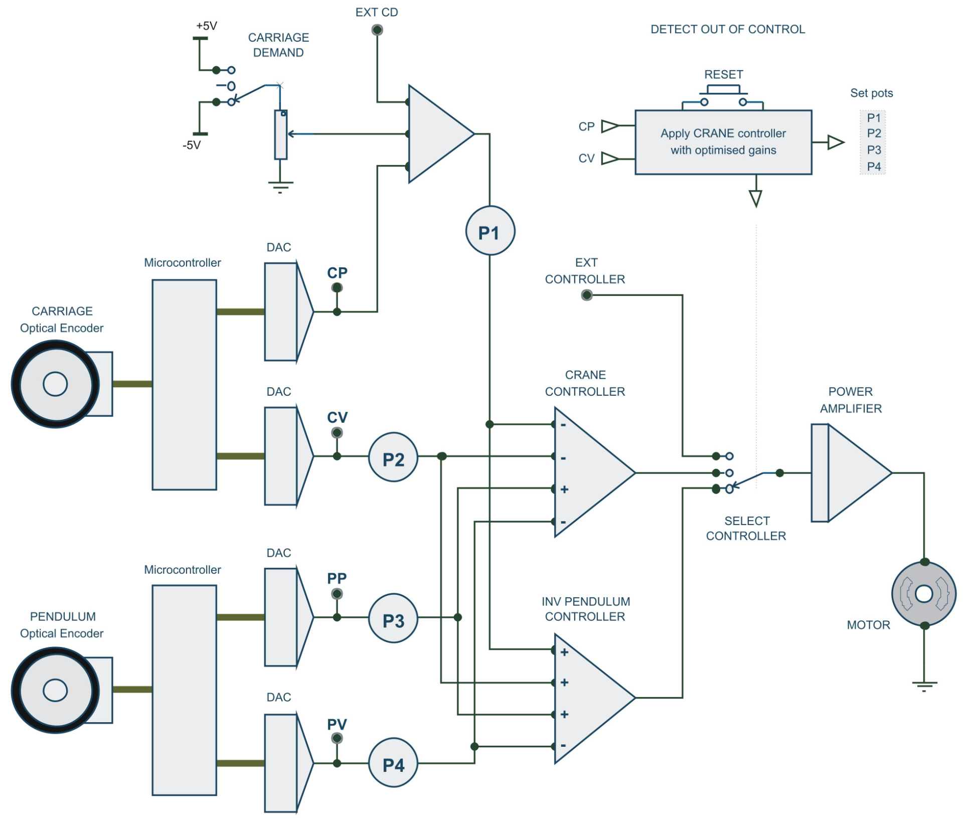 Figure 6: Circuit block diagram for the electrical layout of the system
One important thing to note is that the potentiometers used to set the gains are accurate to 2 decimal places. The calculated gains required to set the poles at the desired locations are likely irrational numbers, and so it is often required to round the gain values to the nearest reachable potentiometer values, and recalculate the theoretical pole locations.
Results and Discussion
Crane
Friction Measurement
The dynamic and static friction were measured as 2.4 and 3.0 N respectively.
Empirical Synthesis of \(p_3\) and \(p_4\) Controller
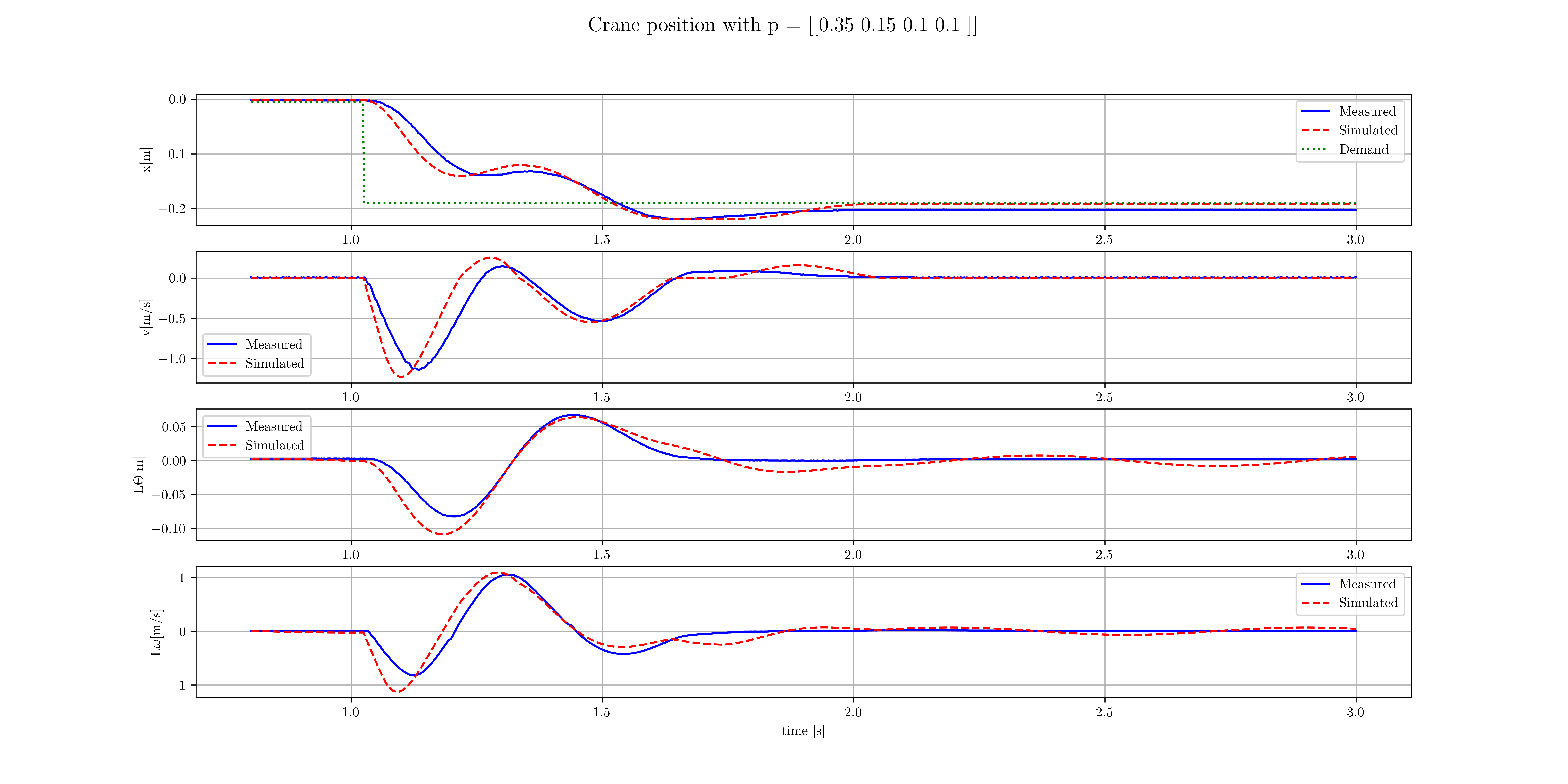 Figure 7: Empirical synthesis of controller gains
From Figure 7 the oscillatory response of the carriage velocity was measured to give a period of 0.36s giving a frequency of 17.45 rad/s. The response also shows moderate damping where the amplitude of carriage velocity halved over about 1 period, giving a damping ratio of \(\zeta \approx 0.11\).
From the closed loop gain setpoints the pole locations are calculated as:
\([-3.8986 \pm 18.693j, -2.1693 \pm 6.4649j]\)
These indicate a highly damped system with frequency responses of 18.7 and 6.5 rad/s and corresponding damping ratios of 0.208 and 0.336.
The frequency is consistent with the calculated pole locations. The measured damping ratio is slightly lower than expected, which is likely due to high uncertainty in the periods over which the amplitude halved, and the rule of thumb method used requiring small damping ratios to be valid.
There is a small discrepancy between the simulated and observed responses. This is due to uncertainty in system parameters rather than numerical error in the verlet integrator method. Uncertainty in the system parameters include the sensor constants, amplifier gains, friction coefficients, mass and moments of inertia of the system.
Pole Placement
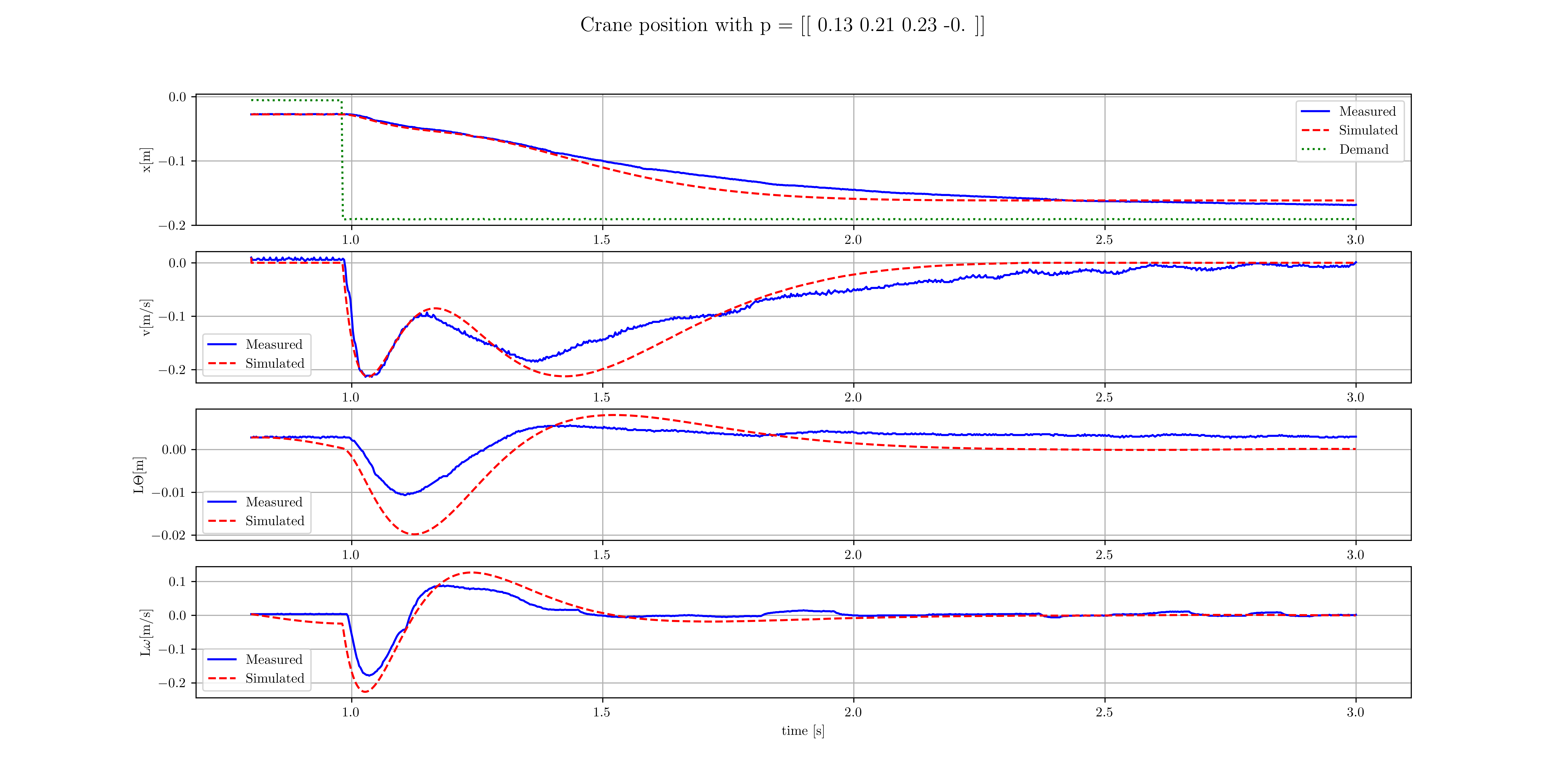 Figure 8: Step response of crane system with feedback gains chosen such that all four poles lie close to \(-\omega_1 = -\sqrt{78.5}\)
The gains were calculated from equating expanded coefficients of \((s - \omega_1)^4\) with the characteristic polynomial. These were found to be \([0.13, 0.21, 0.23, 0.00]\), rounded to 2 decimal places which was the maximum precision of the potentiometers.
The calculated poles from 2 decimal place rounded gain values were found to be \([-12.454 \pm 6.4622j, -4.8908 \pm 2.8411j]\). This shows that the poles are not consistent with the target pole position. Figure 4 demonstrates the high sensitivity of the pole locations to small variations of coefficients in the characteristic polynomial. This explains why the position of the 2 decimal place rounded gains are so far from the target pole positions.
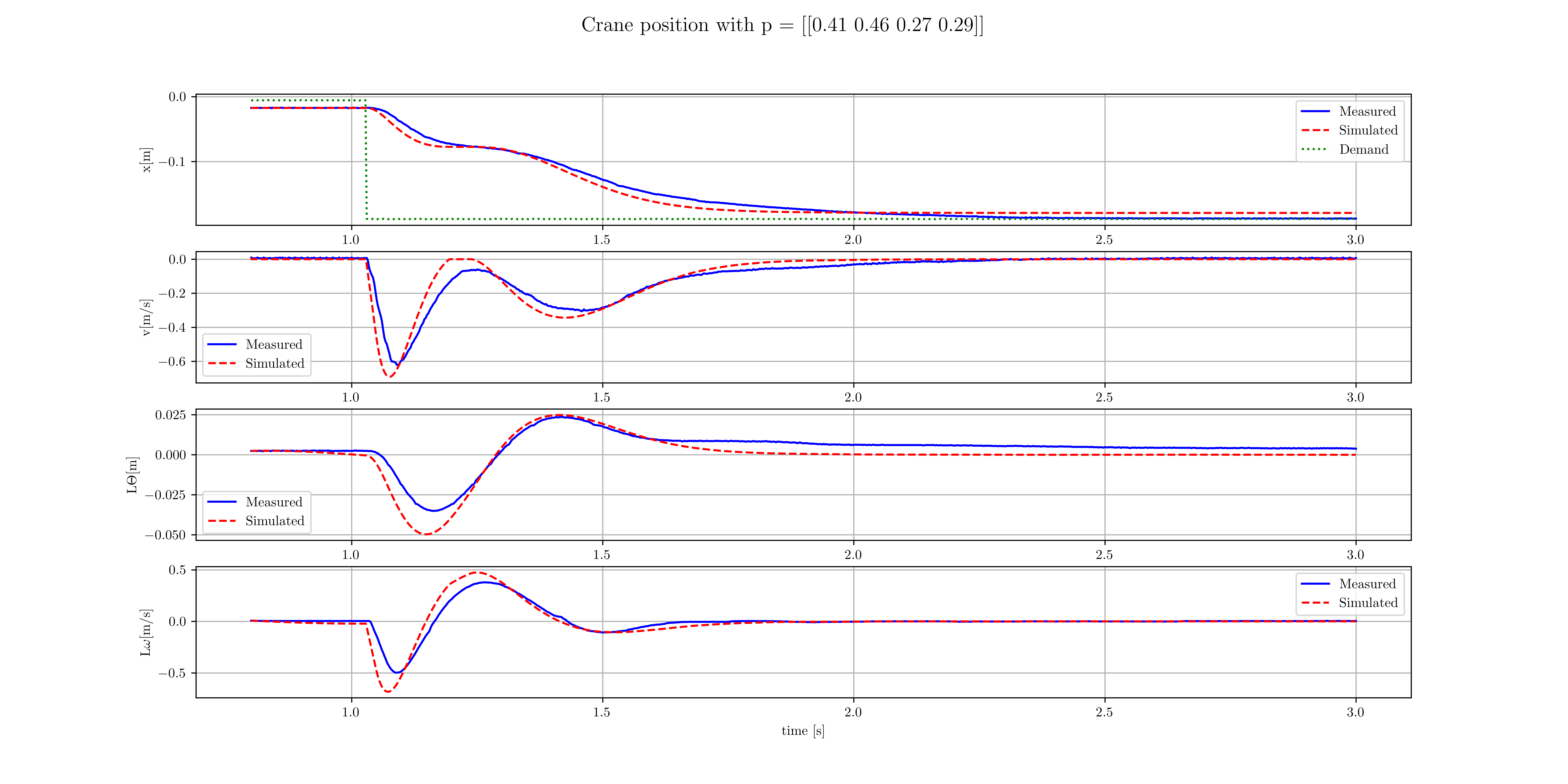 Figure 9: Step response of crane system with feedback gains chosen such that poles lie close to \(-\omega_1\) at \(-\alpha, -\beta, -\omega \pm j\omega\) where \(\alpha = \beta = \omega = 10\)
Figure 9 shows the response for gains calculated at chosen pole locations, \(-\alpha, -\beta, -\omega \pm j\omega\). The values were chosen as \(\alpha = 10; \beta = 10; \omega = 10\) for which the gain values were calculated by expanding the polynomial from the roots and equating coefficients with the characteristic polynomial. These were found to be \([0.4128, 0.4628, 0.2721, 0.2883]\)
The gain values, rounded to 2 decimal places, give poles of \([-10.34 \pm 10.61j, -9.32 \pm 1.91j]\) which is quite close to the design point of a repeated pole at \(-10\), and poles at \(-10 \pm 10j\).
The response shows some oscillation components, but the system is highly damped and the frequency response is difficult to measure. However, it does reach the step demand faster, suggesting that the real part of the poles are further from the imaginary axis than in Figure 7. This makes it difficult to compare the observed response with the pole locations. The response does however closely match the simulated response, given the uncertainty of the system parameters.
Variation of \(p_2\)
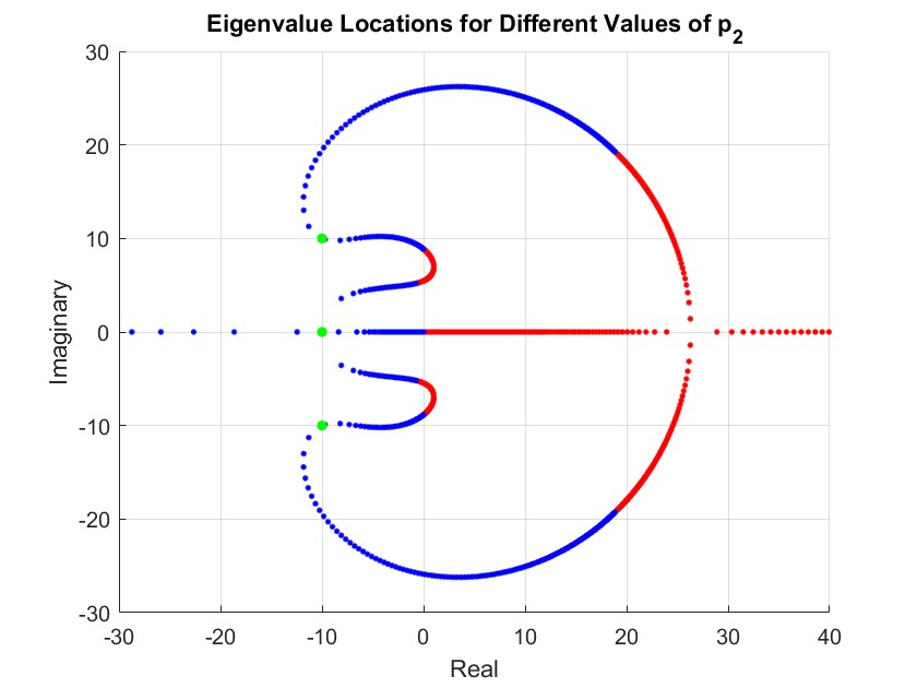 Figure 10: Crane pole positions for varying \(p_2\) only with \(p_1 = 0.4128, p_3 = 0.2721, p_4 = 0.2883\)
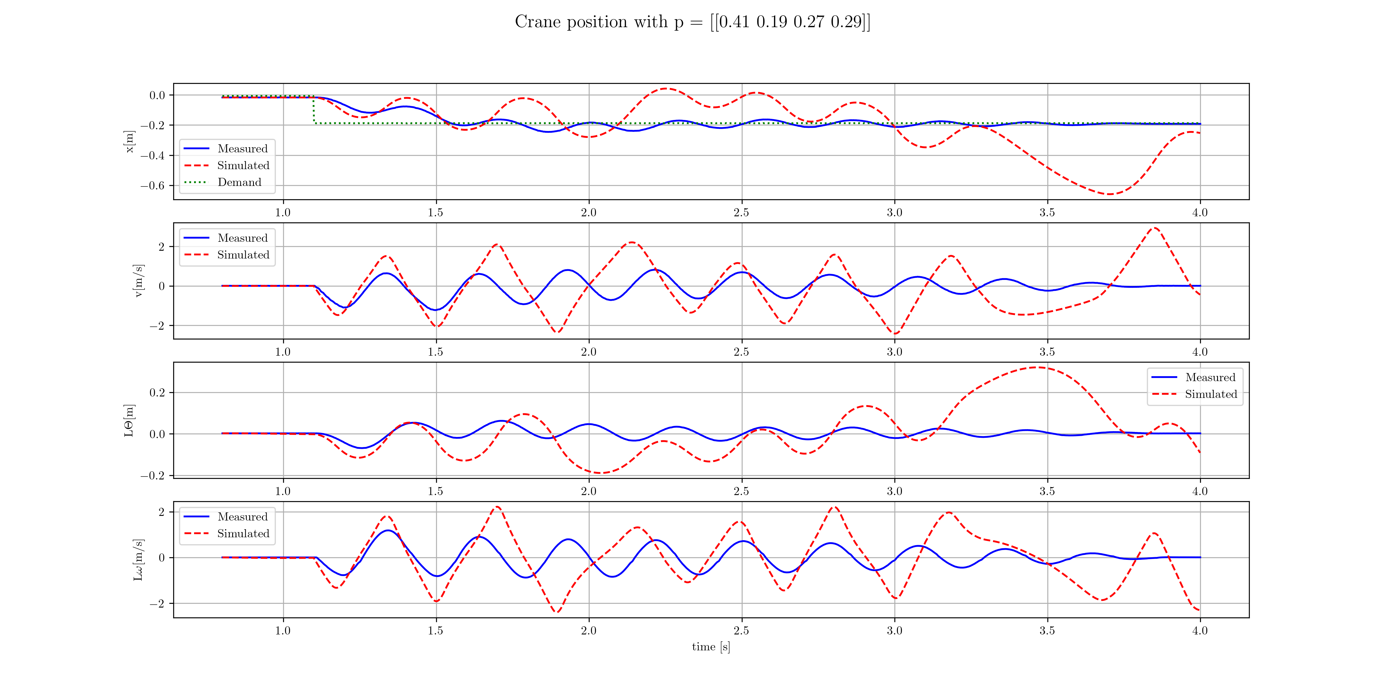 Figure 11: Limit of stability
Figure 10 shows the pole locations of the system as \(p_2\) is varied. As \(p_2\) is increased the pole locations follow the locus around to the right, where they reach the imaginary axis at the limit of stability. The blue shows positive values for \(p_2\) and the red shows negative values. This graphically shows the Routh-Hurwitz criteria for \(k_2 > 0\).
Figure 11 shows the real system’s response at the smallest \(k_2\) where instability starts to occur. The value of \(p_2\) reduced from 0.46 to 0.19 which corresponds to \(k_2 = 31.35\). The measured frequency was 21.67 rad/s and the amplitude of velocity of the carriage dropped to half of the maximum value after 4 cycles, giving the damping ratio as \(\zeta \approx 0.03\).
From the predicted gain equation, the predicted gain at the onset of instability is \(k_2 = 41.43\) and frequency \(\hat{\omega} = 25.76\) rad/s. Additionally, the theoretical closed loop pole locations were found as \([4.5748 \pm 26.112j, -1.9365 \pm 4.9511j]\). The first two poles that lie to the right of the imaginary axis suggests that the system should be unstable for this value of \(p_2 = 0.19\).
Both of these indicate that the lower bound gain \(k_2\) at the onset of instability is smaller than expected. This means that the system is more stable than predicted by the linear model. From nonlinear theory, for oscillations of amplitude \(E\) there is an additional gain \(\Delta k_2\) which is inversely proportional to \(E\). Figure 10 also shows the effect of this additional gain, as it causes the poles to move further to the left of the imaginary axis. For small oscillations the real system has a large additional damping term from friction, which is why the linear model predicts instability to occur at a higher gain than observed. At any smaller gain, the oscillations occur at larger amplitudes which reduces additional damping from friction causing the system to become unstable.
Inverted Pendulum
No Carriage Feedback
For the case where \(p_3 = p_4 = 0\), so no pendulum feedback, then the carriage accelerated away from the set zero position showing instability. A first test showed that even a very small pendulum angle caused an initial motion of the carriage. On another test, the pendulum was carefully left at an initial angle of zero, where it was stationary. A very small force displaced the pendulum and the carriage accelerated away from the zero position. This instability is predicted by the poles of the system, where there is a repeated pole at 0.
Pole Placement
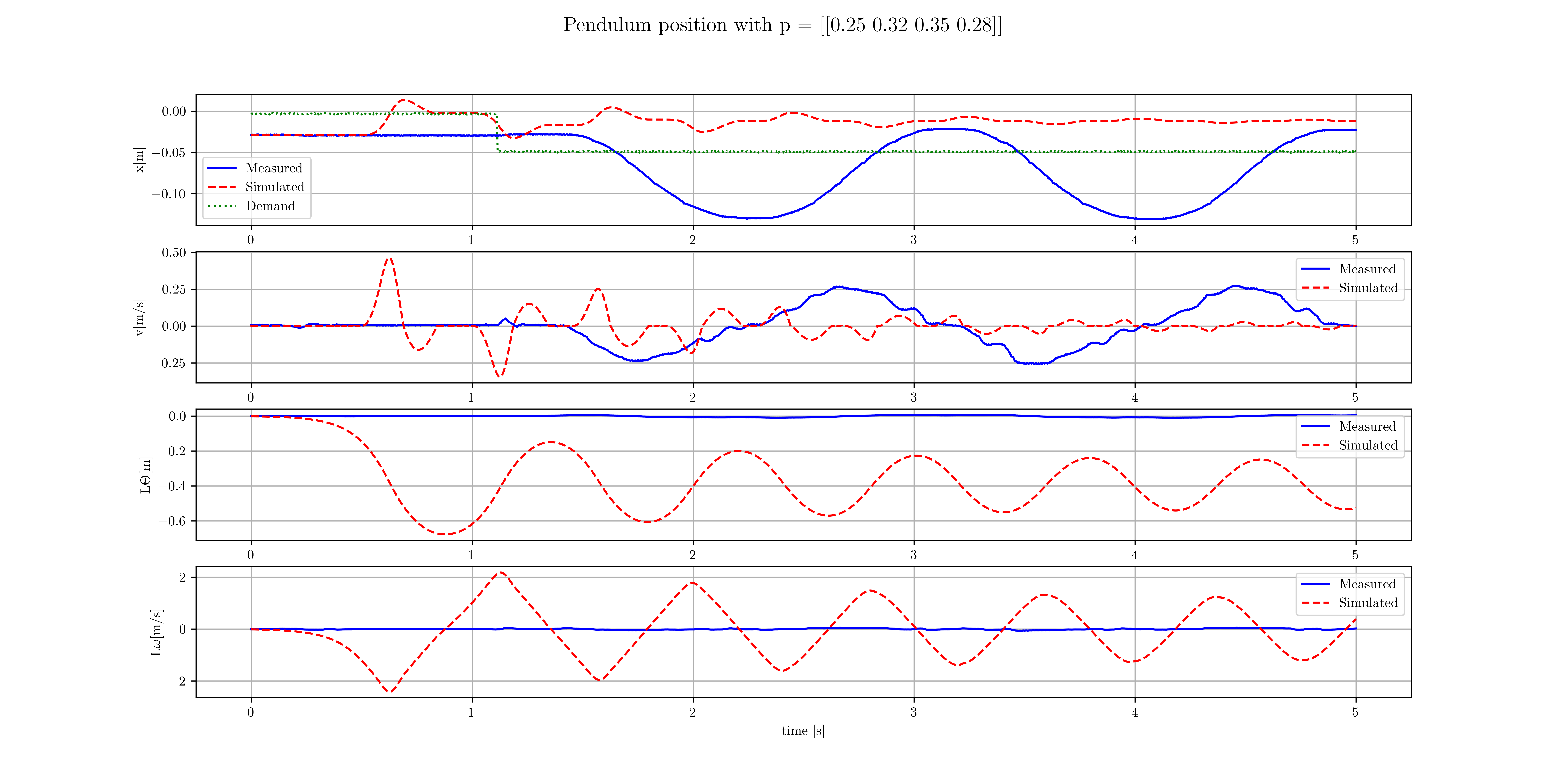 Figure 12: Step response of pendulum system with feedback gains chosen such that all four poles lie close to \(-\omega_1 = -\sqrt{78.5}\)
Figure 12 shows the response of pendulum system with feedback gains chosen such that all four poles lie close to \(-\omega_1 = -\sqrt{78.5}\). These values were found to be:
\(\mathbf{P} = [0.2540, 0.3222, 0.3465, 0.2802]\)
The corresponding poles at the rounded gain values are:
\([-12.3384 \pm 4.907j, -5.439 \pm 2.182j]\)
These poles are not very close to the desired location of \(-\sqrt{78.5}\).
The measured frequency of the carriage response is 3.59 rad/s which lies in the range of the frequency predicted by the poles. Interestingly, the simulated response of the system is unstable and the pendulum falls over. The cause of this is thought to be due to the accumulation of numerical errors in verlet integration due to friction.
Limit Cycles
From theory covered, derivation of Routh-Hurwitz criteria at the limit of stability gives two solutions for the gain \(k_2\). The first solution corresponds to a low frequency cycle at 2.46 rad/s at a gain of \(k_2 = -7.24\). The second solution corresponds to a higher frequency of 31.63 rad/s at a gain of \(k_2 = -93.8\). Figure 13 shows the pole positions of the system as \(k_2\) is varied. The high frequency case is indicated by where the outer circle crosses the imaginary axis. Similarly, the low frequency case is indicated by where the inner circle crosses the imaginary axis.
The simulated response of the non-linear system for both limit cycles is unstable and the pendulum falls over. Reasons for this are not fully understood, but it is likely due to the external friction forces. Verlet integration should conserve energy, however with large components of external friction in the limit cases, numerical error may accumulate.
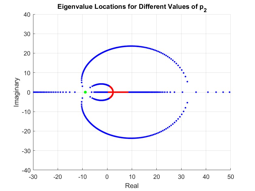 Figure 13: Pendulum pole positions for varying \(p_2\) only with \(p_1 = 0.23, p_3 = 0.63, p_4 = 0.40\)
The red poles are where \(p_2 < 0\) for which the system is unstable. For the outer blue loop, at the imaginary axis the poles are at the high frequency limit cycle. As \(k_2\) increases, becoming less negative, the poles move to the left and become more damped.
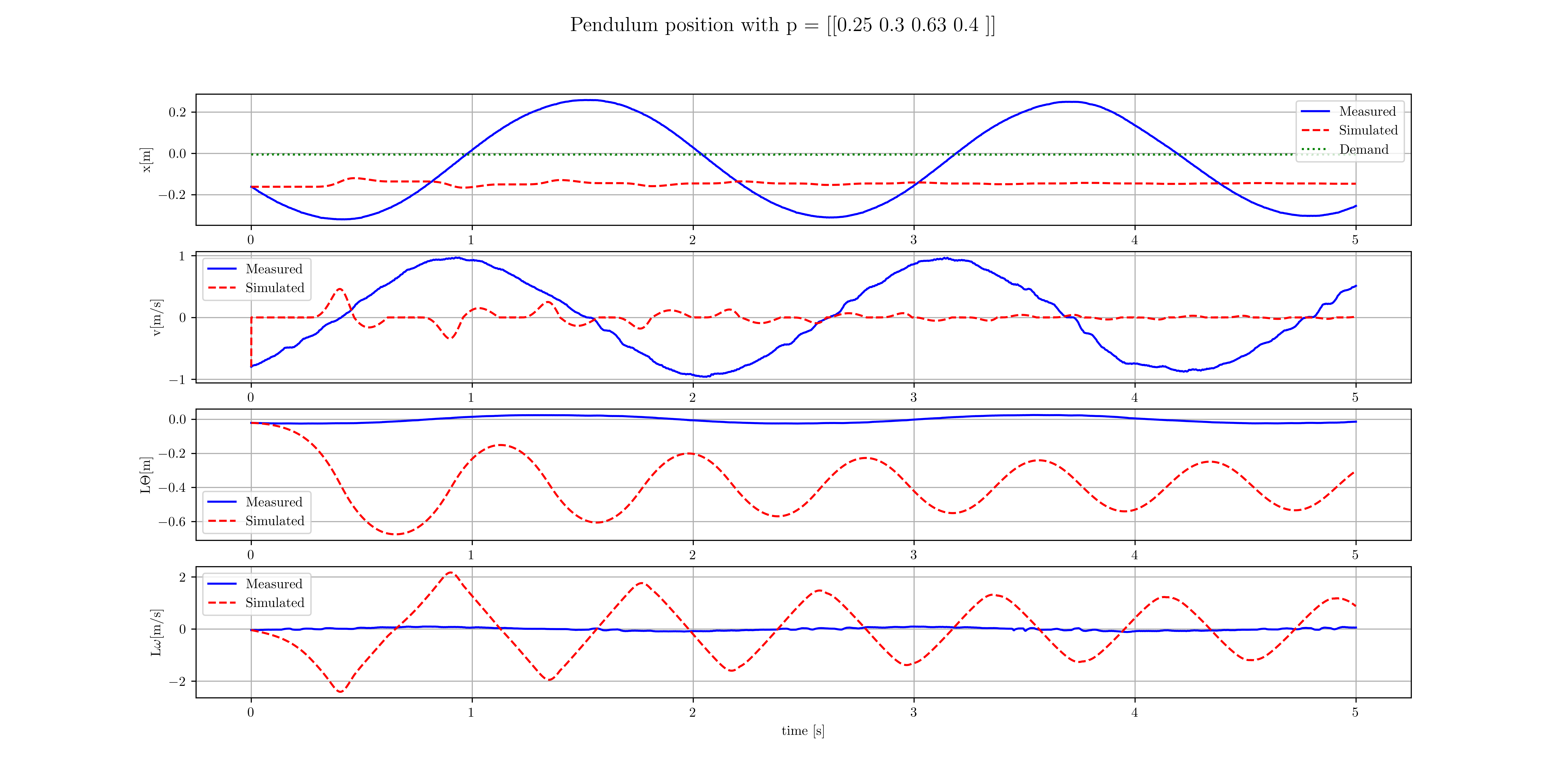 Figure 14: Inverted pendulum response at minimum set \(k_2\) for stability
Figure 14 shows the actual response at the onset of instability at a lower bound of \(p_2 = 0.30\) which corresponds to \(k_2 = -33.0\). Large oscillations were observed of constant amplitude at a measured frequency of 2.92 rad/s. The frequency is similar to the pole locations \(-1.2703 \pm 2.3783j\) and to the low frequency limit cycle frequency \(\hat{\omega} = 2.46\) rad/s. The observed damping ratio is much lower than predicted by the poles, which suggests the magnitude of \(k_2\) is much smaller.
From nonlinear theory, for oscillations of amplitude \(E\) there is an additional gain \(\Psi(E)\) which is inversely proportional to \(E\). At the limit for stability the overall gain, \(k_2 + \Psi(E) = k_{2,\text{crit}}\), where the critical value of \(k_2\) is defined in the previous equation. The reduction in \(k_2\) from the value predicted by linear theory that causes instability is denoted \(\Delta k_2\). The amplitude of oscillations can be calculated as: \[E = \frac{4F}{\pi(M + I/a^2)\Delta k_2}\]
The value of \(E/\hat{\omega}\) was calculated to be 0.117 which is much smaller than the observed, approximately 0.3 m. This suggests from non-linear theory that a smaller value of \(k_2\) should have been achieved. This may not be true however, as the theory perhaps incorrectly assumed that the system filtered out high frequency components of the non-linearity.
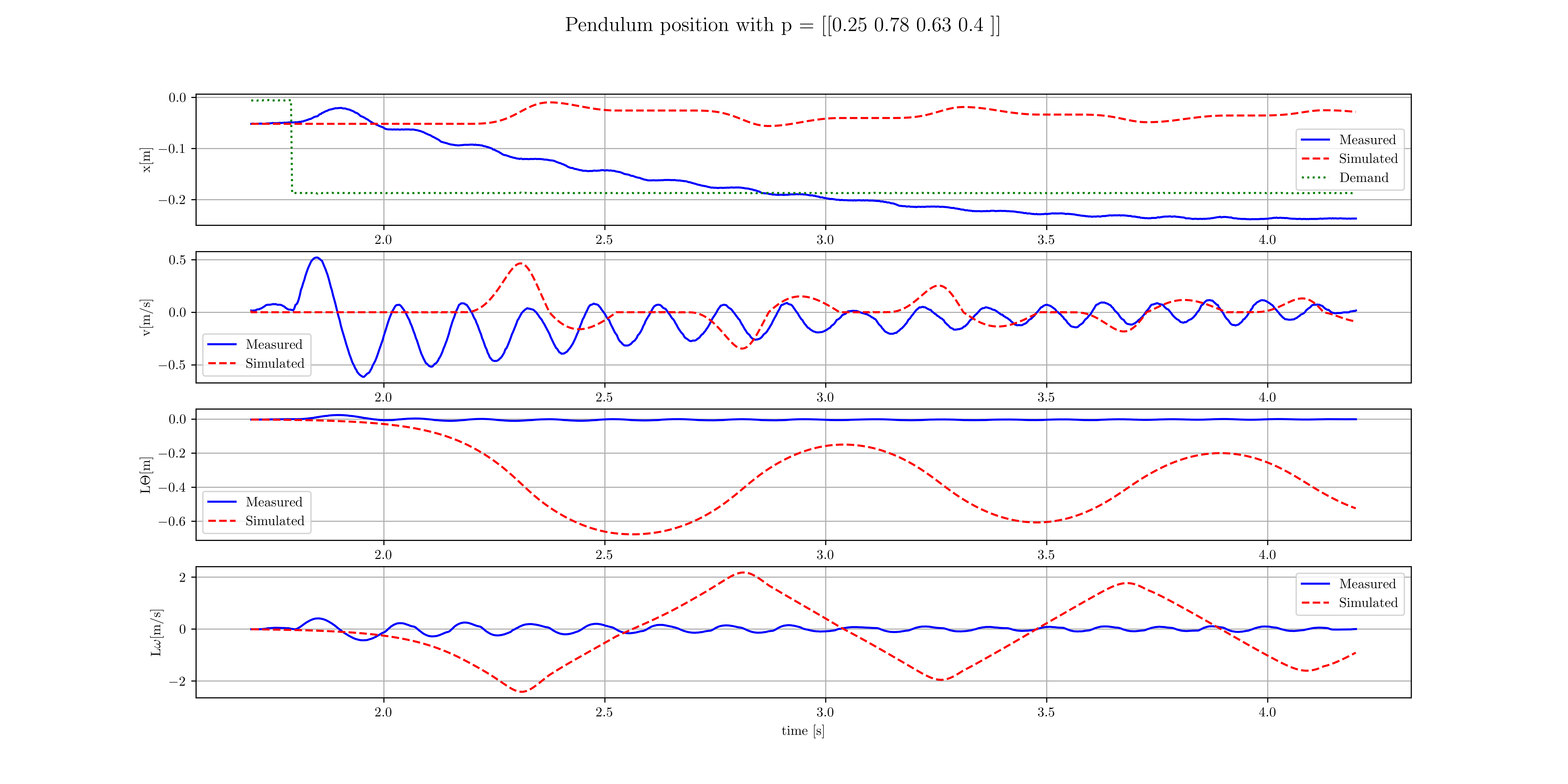 Figure 15: Inverted pendulum response at maximum set \(k_2\) for stability
Figure 15 shows the response at the onset of instability at an upper bound of \(p_2 = 0.78\) which corresponds to \(k_2 = -85.8\). The carriage velocity amplitude halves after approximately 7 cycles which gives a damping ratio of \(\zeta \approx 0.016\). The predicted poles from the closed loop system are \(-4.0715 \pm 30.430j\), giving a damping ratio of 0.1337 which is significantly higher than the measured value.
The frequency of carriage velocity is calculated to be about 44 rad/s, indicating that it’s at the high frequency limit cycle. For small oscillations the additional gain from nonlinearity, \(\Psi(E)\), is positive compared to the negative set value of \(k_2 = -85.8\). The sum of these gives the overall gain a smaller magnitude than the critical \(k_2 = -93.8\), causing the damping ratio to be lower than expected. This also indicates that this Routh-Hurwitz condition is likely not broken, however the system still becomes unstable so another condition must be violated.
No Pendulum Feedback
For the case of no pendulum position or velocity feedback, then \(p_3 = p_4 = 0\). It is already clear that these no longer satisfy the Routh-Hurwitz conditions. With the same \(p_1\) and \(p_2\) values as section 4.2.2 the closed loop poles are calculated as:
\([37.963, 8.5190, -2.0332, -9.2094]\)
Clearly, the poles lie to the right of the imaginary axis indicating that the system is unstable. This is due to positive feedback from the carriage position and velocity shown in the controller layout in Figure 6. This is different to the crane control system as that uses negative feedback to stabilise the carriage. Therefore, the pendulum will fall over, displacing the carriage, and accelerate away from the setpoint.
Inverted Pendulum LQR
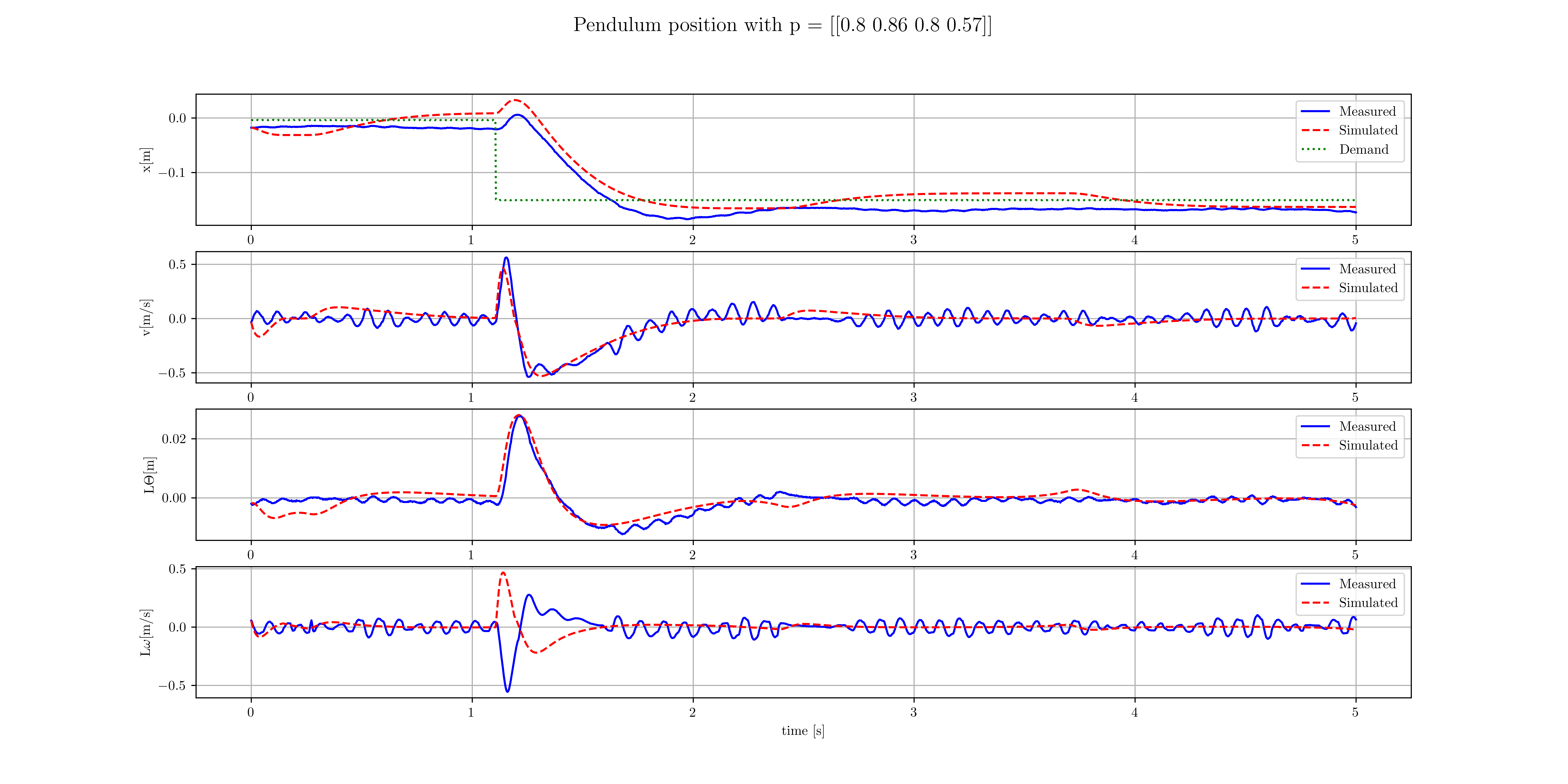 Figure 16: Fast response of the pendulum with LQR
The weighting matrices used were: \[\mathbf{Q} = \begin{bmatrix} 6.25 & 0 & 0 & 0\\ 0 & 0.0001 & 0 & 0\\ 0 & 0 & 58.36 & 0\\ 0 & 0 & 0 & 0.0064 \end{bmatrix} \quad \mathbf{R} = \begin{bmatrix} 0.0001025 \end{bmatrix}\]
From Figure 16 there exist clear oscillations at a frequency of 75.4 rad/s. The pole locations from rounded gains are \([-20.691 \pm 19.306j, -4.0153 \pm 2.8415j]\). The frequency of the small amplitude oscillations differ significantly from the pole frequencies. Additionally, these oscillations are not present in the simulated non-linear response of the system. This suggests that they are caused by noise and the high derivative gain values chosen by LQR.
A higher input signal weight \(\mathbf{R}\) was tested, which produced larger gains and a faster response, however the oscillations grew in amplitude. For further improvement of response times without increasing amplified noise, an observer could be designed to better estimate the derivative states.
Conclusion
In this report, the dynamics of an inverted pendulum system were derived and linearized about both a stable crane and an unstable inverted pendulum equilibrium. State feedback and pole placement techniques were successfully utilized to design controllers for both arrangements. In the crane limit cycle for \(k_2\), the onset of instability occurred at a smaller gain \(k_2\) than predicted by the linear model and Routh-Hurwitz. The describing function for nonlinear signum friction explained this as an additional \(k_2\) gain inversely proportional to oscillation amplitude.
Pole placement was used to shape the system response, though high sensitivity to gains was observed, especially for the cases of repeated poles. For the inverted pendulum, instability was observed for cases of no carriage feedback and no pendulum feedback which agreed with predictions from Routh-Hurwitz criteria and pole placement. High and low frequency limit cycles were observed for the inverted pendulum at minimum and maximum \(k_2\) respective gains. Discrepancy between behaviour predicted by linear theory and observed behaviour was attributed to additional gain from the describing function.
LQR was used to design a controller for the inverted pendulum, which produced a fast response from high gains which made it sensitive to noise, producing high frequency oscillations.
References
- G. Vinnicombe, Inverted Pendulum Lab Handout. University of Cambridge, 2022.
- G. F. Franklin, J. D. Powell, A. Emami-Naeini, Feedback Control of Dynamic Systems. Pearson, 2015.
- H. K. Khalil, Nonlinear Systems. Pearson, 2002.
- R. C. Dorf, R. H. Bishop, Modern Control Systems. Pearson, 2016.
