Heat Exchanger
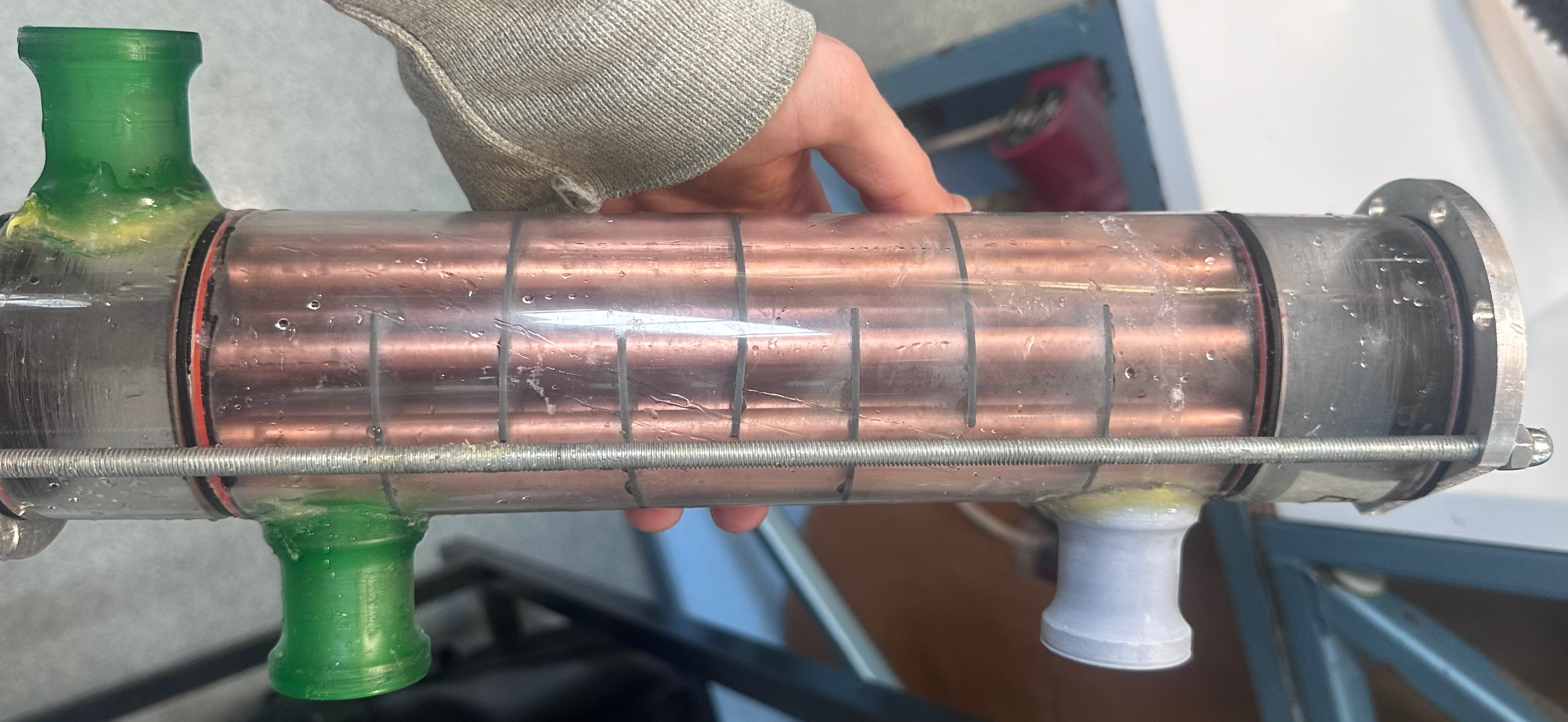
This page is an overview of my project report.
This report presents the development of a software tool to help solve constrained design optimization of a shell and tube heat exchanger. The software is developed in Python and uses LMTD and NTU methods to solve for the output parameters. Computational model is compared with experimental data Various optimization algorithms were tested with constraints and the results are presented.
- Introduction
- Performance Characterisation
- Optimization Problem
- Software
- Software Summary
- Performance degredation
- Performance Comparison
- Uncertainty
- Group results
- Design recommendations
- Conclusion
- Group Photo
Introduction
Heat exchangers have a wide range of applications in HVAC, power generation and chemical industries. These essential components are typically much larger than other components in a system and can significantly contribute to the overall cost. Designing high performance, low cost heat exchangers involves solving complex optimization problems with multiple constraints. The software is developed in Python and implements Kerns, LMTD and NTU methods to solve for heat exchanger performance.
Objectives
To analyse pressure loss and heat transfer for various shell and tube heat exchanger designs.
To produce a software tool for constrained design optimization of shell and tube heat exchangers.
To select an optimal design to be compared with other groups designs and software tools.
To manufacture and test the selected design against other groups and software predictions.
Performance Characterisation
Hydraulic Analysis
The pressure drop across for each section of the heat exchanger can be calculated from the mass flow rate and the geometry of the components through empirical relations. The compressor characteristics in the closed loop circuit relate the equivilent pressure drop for a given mass flow rate. This is iteratively solved to calculate the mass flow rate for a heat exchanger design and compressor characteristic.
The pressure drop in shell side flow is more complex than the tube side flow due to bundle pass and baffle configurations. Kerns method was used to calculate the pressure drop in each cold flow pass. This uses an effective diameter which depends on triangular or square pitch and a bundle crossflow area.
Thermal Analysis
LMTD and $\mathcal{E}$-NTU methods were used to calculate the heat transfer rate from the mass flow rates found in the hydraulic analysis. Both methods require an overall heat transfer value $HA$ which is calculated from tube geometry, film heat transfer coefficients and tube conductivity. Kerns method is used to calculate the shell side film heat transfer coefficient $h_o$ from terms defined in the hydraulic analysis.
\(\mathcal{E}\)-NTU
The \(\mathcal{E}\)-NTU method is used to calculate the heat transfer rate for a wide range of heat exchanger configurations. The effectiveness can be found from a dimensionless number of "transfer units" denoted \(NTU\) and a heat capacity rate ratio, \(C^*\) or \(R\). The \(\mathcal{E}\)-NTU method changes when the shell fluid is minimum or maximum heat capacity rate. A generalised method known as P-NTU defines a temperature effectiveness \(P\) as a function of NTU and a ratio of heat capacity rates \(R\) both defined below. \[NTU = \frac{HA}{C_{\text{min}}} \quad , \quad R_1 = \frac{C_1}{C_2} \quad , \quad P_1 = \frac{C_\text{min}}{C_1} \mathcal{E} = f(NTU, R_1)\]
Extensive work has been done to find functions, \(f\), for various heat exchanger configurations to calculate \(P\), and hence \(\mathcal{E}\) [1]. This can then used to obtain outlet temperatures and heat transfer rate \(\dot{Q}\).
LMTD
The Log Mean Temperature Difference (LMTD) method is based on the analytical solution for a single stage counterflow heat exchanger. For a general heat exchanger, a correction factor $F$ is applied which represents the deviation from counterflow log mean temperature difference. \[\dot{Q} = HAF \Delta T_{\text{lm}} \quad \text{where} \quad \Delta T_{\text{lm}} = \frac{\Delta T_1 - \Delta T_2}{\ln(\Delta T_1 / \Delta T_2)}\]
For this counterflow definition of F, \(\Delta T_1 = T_{\text{hot,in}} - T_{\text{cold,out}}\) and \(\Delta T_2 = T_{\text{hot,out}} - T_{\text{cold,in}}\). Variations from this, including the coflow case or multiple passes, require the F factor to be calculated from the P-NTU temperature effectiveness, \(P_1\), and heat capacity rate ratio \(R_1\) from well defined relations [1].
Optimization Problem
The goal is to maximise the heat transfer rate \(\dot{Q}\) subject to physical constraints. Many standard physical quantities are constrained to discrete values and standards, such as the number of tubes, baffles and tube diameters. For our design, we have the following constraints:
Total mass of the heat exchanger \(M < 1.2\) Kg.
Total length of the heat exchanger \(L_{\text{total}} < 0.35\) m.
Total length of the tubes \(\sum L_{\text{tube}} < 3.5\) m.
Tubes have outer and inner diameters, \(d_{o} = 8\) mm, and $d_{i} = 6$ mm.
Shell has inner diameter \(D_{\text{shell}} = 64\) mm.
Nozzles must not be closer than \(20\) mm to the edge of the shell or header end.
The tube pitch must be greater than \(12\) mm.
The mass calculation has a level of uncertainty in the manufactured components and so the constraint is reduced to 1.1 kg. The total length of the tubes constraint must be modified to account for the manufacturing process. For \(n_t\) total tubes, \(n_t - 1\) cuts with a blade thickness of \(1.5 mm\) are required and so the actual maximum length is given below. \(\sum L_\text{tube} < 3.5 - 0.0015 \times (n_t - 1)\) The tube lengths are also limited by the maximum length of the heat exchanger, $0.35$ m. The nozzle width is 40 mm, however, if there is an even number of hot sections then the nozzles are on the same side so the opposite end section can be shortened. This can allow a longer maximum tube length than an odd number of hot passes. \(L_\text{tube} < 0.29 - 0.02 \times ( N_{hot}\mod 2)\) Additional constraints were also imposed to reduce the search space and simplify the problem.
The number of baffles was constrained to 8 in the cold fluid path. This was also to prevent the baffle spacing to become small relative to the shell diameter and cause further innacuracies in Kerns method.
The number of tubes was constrained to not decrease over the hot fluid path inside the heat exchanger. This should not exclude the global optimium because increasing the area at regions of smaller temperature difference increases overall heat transfer. For example, if we allowed the area to decrease then more heat transfer would occur in the first stage, however there would be a significant reduction of heat transfer in the later stages from both reduced area and temperature difference.
Algorithms
Three optimization algorithms were tested: Brute force, Sequential Least Squares Programming, and Simplicial Homology Global Optimization. The Simplicial Homology Global Optimization algorithm was chosen for its robustness and ability to find optima in all cases. SHGO is a derivative-free global optimization algorithm that efficiently subdivides the search space into smaller regions (simplicial complexes) to find the global optimum [3].
Software
Implementation
The Python application used PyQt6 and matplotlib for the GUI. The calculations were done using NumPy and SciPy libraries. The software tool allows the user to interactively change the design parameters for a wide range of heat exchanger configurations. Calculated values are displayed in real-time and the user can compare the performance of different designs. The software features object oriented design with classes for the heat exchanger and fluid path components. The structure is designed to easily modify fluid properties and introduce new flow components. Seperate optimization threads are used to prevent the GUI from freezing during long calculations. A log displays optimization progress, warning and error messages. There is also a diagram of the heat exchanger which helps the user visualise the flow path of multi-stage designs.
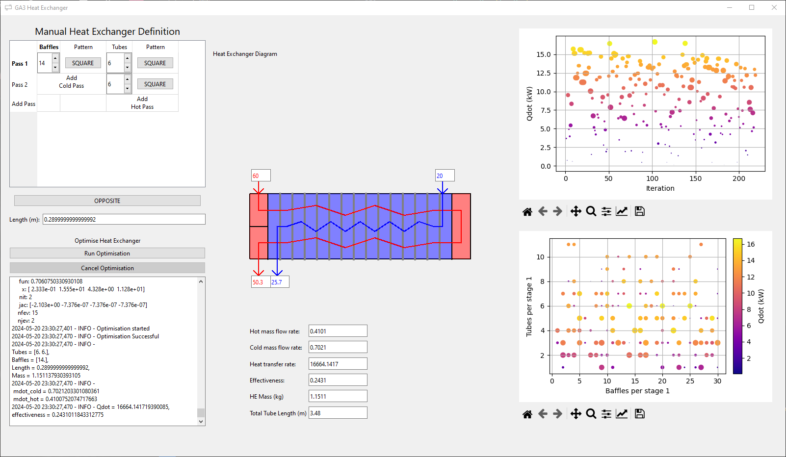 {#fig:software width=”60%”}
Best Designs from Constraints
| \(N_\text{cold}\) | \(N_\text{hot}\) | Pattern | Tubes | Baffles | \(L_\text{tube}\) | \(\dot{m}_1\) | \(\dot{m}_2\) | \(\dot{Q}\) | \(\epsilon\) | Mass | \(\Sigma L_\text{tube}\) |
|---|---|---|---|---|---|---|---|---|---|---|---|
| 1 | 1 | Triangle | 13 | 8 | 0.2678 | 0.5892 | 0.4778 | 12297 | 0.1446 | 1.095 | 3.482 |
| 1 | 1 | Square | 13 | 8 | 0.2678 | 0.5885 | 0.4778 | 12314 | 0.145 | 1.095 | 3.482 |
| 1 | 2 | Triangle | 6,6 | 8 | 0.2877 | 0.5928 | 0.4296 | 14126 | 0.211 | 1.100 | 3.452 |
| 1 | 2 | Square | 6,6 | 8 | 0.2877 | 0.5928 | 0.4296 | 14123 | 0.2109 | 1.100 | 3.452 |
| 1 | 3 | Triangle | 4,5,5 | 8 | 0.2470 | 0.5818 | 0.3685 | 14328 | 0.2524 | 1.079 | 3.481 |
| 1 | 3 | Square | 5,5,5 | 8 | 0.2320 | 0.5755 | 0.3855 | 14336 | 0.2414 | 1.076 | 3.479 |
| 2 | 2 | Triangle | 5,6 | 8,8 | 0.2900 | 0.5908 | 0.4174 | 13896 | 0.2106 | 1.085 | 3.190 |
| 2 | 2 | Square | 6,6 | 8,7 | 0.2766 | 0.5902 | 0.4304 | 13901 | 0.2044 | 1.100 | 3.319 |
| 2 | 4 | Triangle | 4,4,4,4 | 7,7 | 0.2173 | 0.5714 | 0.3209 | 14136 | 0.2828 | 1.091 | 3.478 |
| 2 | 4 | Square | 4,4,4,4 | 7,7 | 0.2173 | 0.5728 | 0.3209 | 14103 | 0.2816 | 1.091 | 3.478 |
Optimized Designs for a variety of heat exchanger configurations, with the limiting constraint in bold.
It was interesting to see that the software tool was finding longer solutions with additional tubes in later hot passes over shorter designs with an equal number of tubes in each hot pass. However, this design with a different number of tubes in each section is much harder to manufacture than a circularly symmetric design.
From table 1{reference-type=”ref” reference=”table:designs”} the yellow row shows the optimal design predicted by the software has 1 cold stage and 3 hot stages. This was the design proposed by our pair and selected by the group. During the development of CAD, slight modifications were made and checked with the software tool. A slightly shorter 5,5,5 tube configuration was used for circular and axial symmetry, reducing the number of unique components and simplifying the manufacturing process. The group also decided to reduce the number of baffles to 7. This may have been out of concern that the baffle spacing would become too small relative to the shell diameter. There are also practical reasons for having an odd number of baffles, as the cold inlet and outlet nozzles are on the same side of the shell.
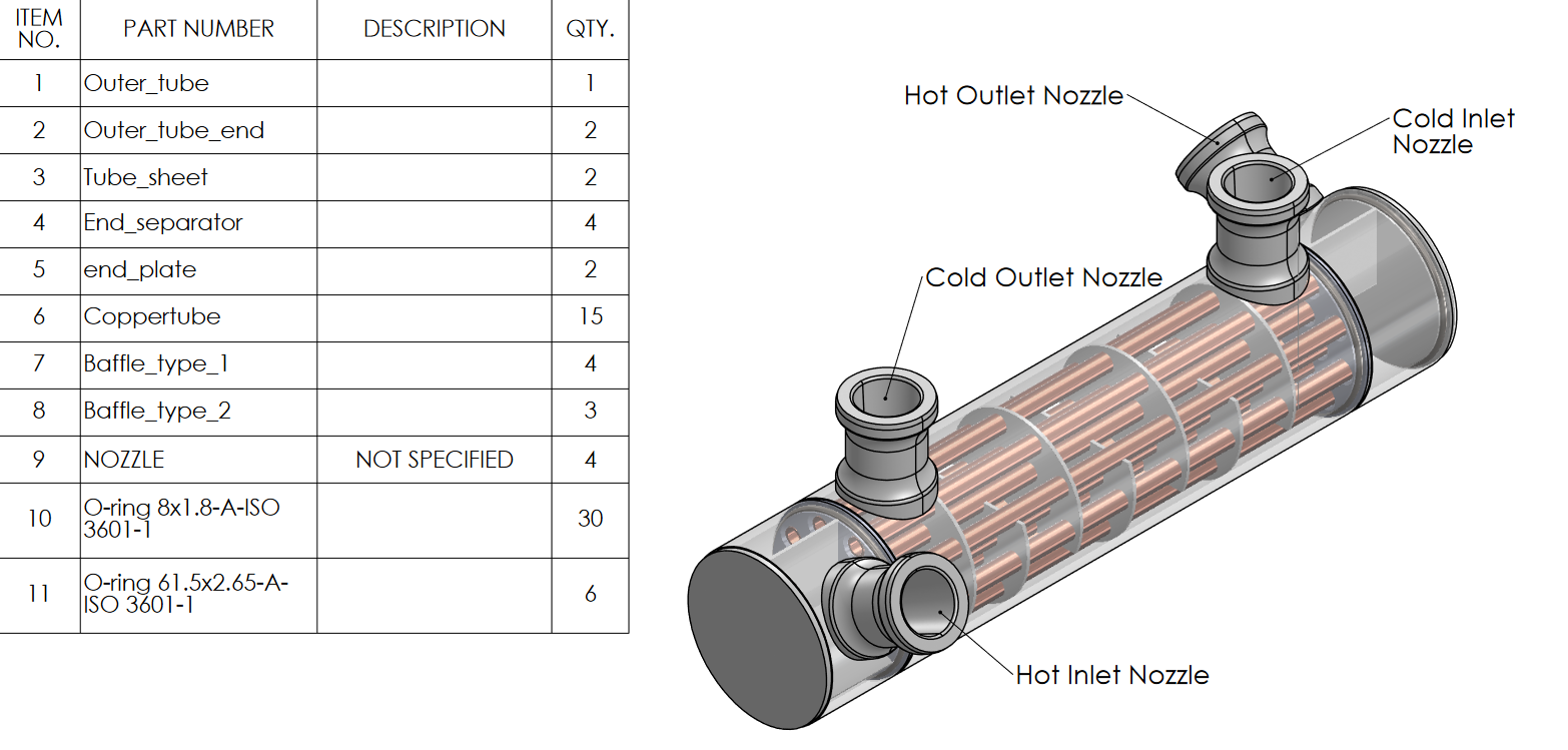 {#fig:final_design width=”85%”}
Software Summary
Hydraulic analysis was performed using Kerns method and compared with experimental data. Innacuracies in the method were identified for the cold flow path and improved by a linear fit to the pressure calculation. \(\mathcal{E}\)-NTU and LMTD methods were compared by calculation time, with \(\mathcal{E}\)-NTU being 2-2.5 times faster on average. Calculated heat transfer rates showed a strong correlation of \(\mathbf{0.91772}\) to experimentally measured values for a range of heat exchanger designs. An interactive software tool was developed to rapidly test a wide range of heat exchanger configurations and compare performance. Common mass and geometry specification constraints were considered with further constraints to reduce the search space. Three algorithms for finding an optimal design were compared and SHGO was chosen for its robustness and ability to find optima in all cases. Various heat exchanger configurations were optimised for which were limited by different constraints. The highest heat transfer design with 1 cold stage and 3 hot stages was selected and small design modifications were made for manufacturability.
Performance degredation
Performance degredation due to fouling is also considered but only the results are shown here.
Performance Comparison
There were small modifications made to the software for some groups unique designs.
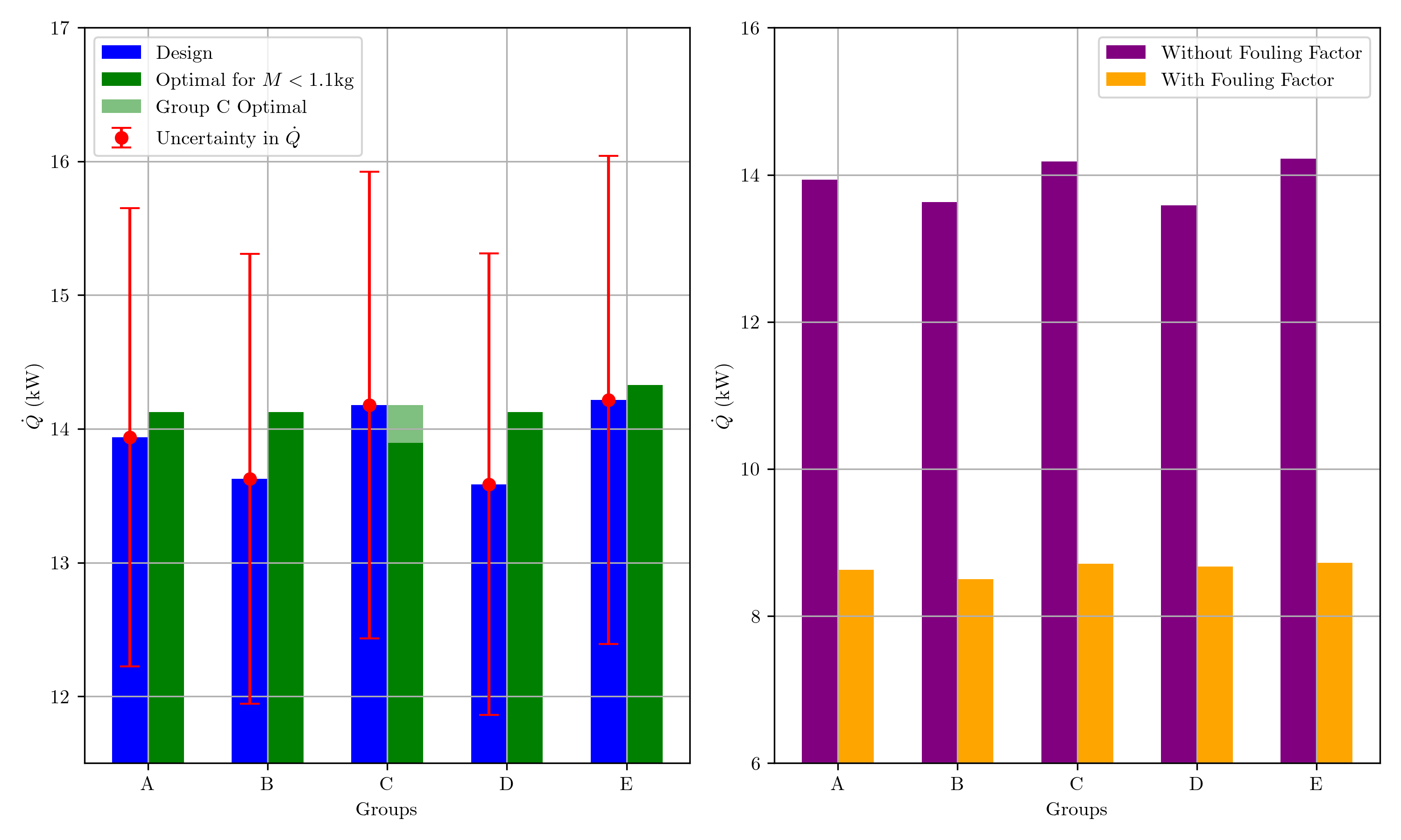 {#fig:2024_performance width=”80%”}
Uncertainty
The following is significantly simplified from the report.
Uncertainty in heat transfer rate was propagated from a central difference derivative. Uncertainty in pitch was estimated from the difference in calculated and a "true average" value. The values \(u_\text{cold}(\dot{Q})\) and \(u_\text{hot}(\dot{Q})\) represent uncertainty over the whole compressor characteristics. The uncertainty in the fit to previous data is also considered with a 90\% confidence interval.
| Group | \(u_Y(\dot{Q})\) (%) | \(u_L(\dot{Q})\) (%) | \(u_{T_\text{1in}}(\dot{Q})\) (%) | \(u_{T_\text{2in}}(\dot{Q})\) (%) | \(u_\text{cold}(\dot{Q})\) (%) | \(u_\text{hot}(\dot{Q})\) (%) | \(u_\text{unc}(\dot{Q})\) (%) | \(u_\text{cor}(\dot{Q})\) (%) |
|---|---|---|---|---|---|---|---|---|
| Group-A | 2.384050 | 0.119312 | 1.348202 | 1.348202 | 0.718815 | 1.257291 | 3.380932 | 12.30 |
| Group-B | 2.307477 | 0.127439 | 1.322163 | 1.322163 | 0.690370 | 1.243790 | 3.295534 | 12.35 |
| Group-C | 2.437940 | 0.116954 | 1.367768 | 1.367768 | 0.726736 | 1.266629 | 3.439666 | 12.31 |
| Group-D | 3.174105 | 0.132264 | 1.318523 | 1.318523 | 0.714964 | 1.235442 | 3.950561 | 12.69 |
| Group-E | 3.860030 | 0.137442 | 1.371735 | 1.371735 | 0.735290 | 1.162906 | 4.535972 | 12.84 |
{reference-type="ref" reference="tab:uncorrected_uncertainty"}](/assets/img/projects/heat_exchanger/Qdot_result_bands.png) {#fig:uncertainty_regions width=”99%”}
{#fig:uncertainty_regions width=”99%”}
The performance of the 2024 designs is shown in figure 3{reference-type=”ref” reference=”fig:2024_performance”}. With little confidence, our software predicts that our design will perform the best out of all groups. It can also be seen that despite small manufacturing modifications made to our design, it is still close to the optimal found. Group C’s design was predicted to come 2nd with a heat transfer 0.28% below our design. Their design was calculated to be much heavier at 1.145 kg, which does not accurately include the weight of the manifold. A seperate optimisation was performed with a relaxed mass constraint, which agreed that group C’s design was the closest to optimal. In third place was group A, with a heat transfer 1.97% below our design. This was 1.34 % below predicted optimal for their configuration. Groups B and D were predicted at 4th and 5th place respectively, with heat transfers 4.15% and 4.44% below our design. These were also 3.53% and 3.82% below predicted optimal for their configurations.
Group results
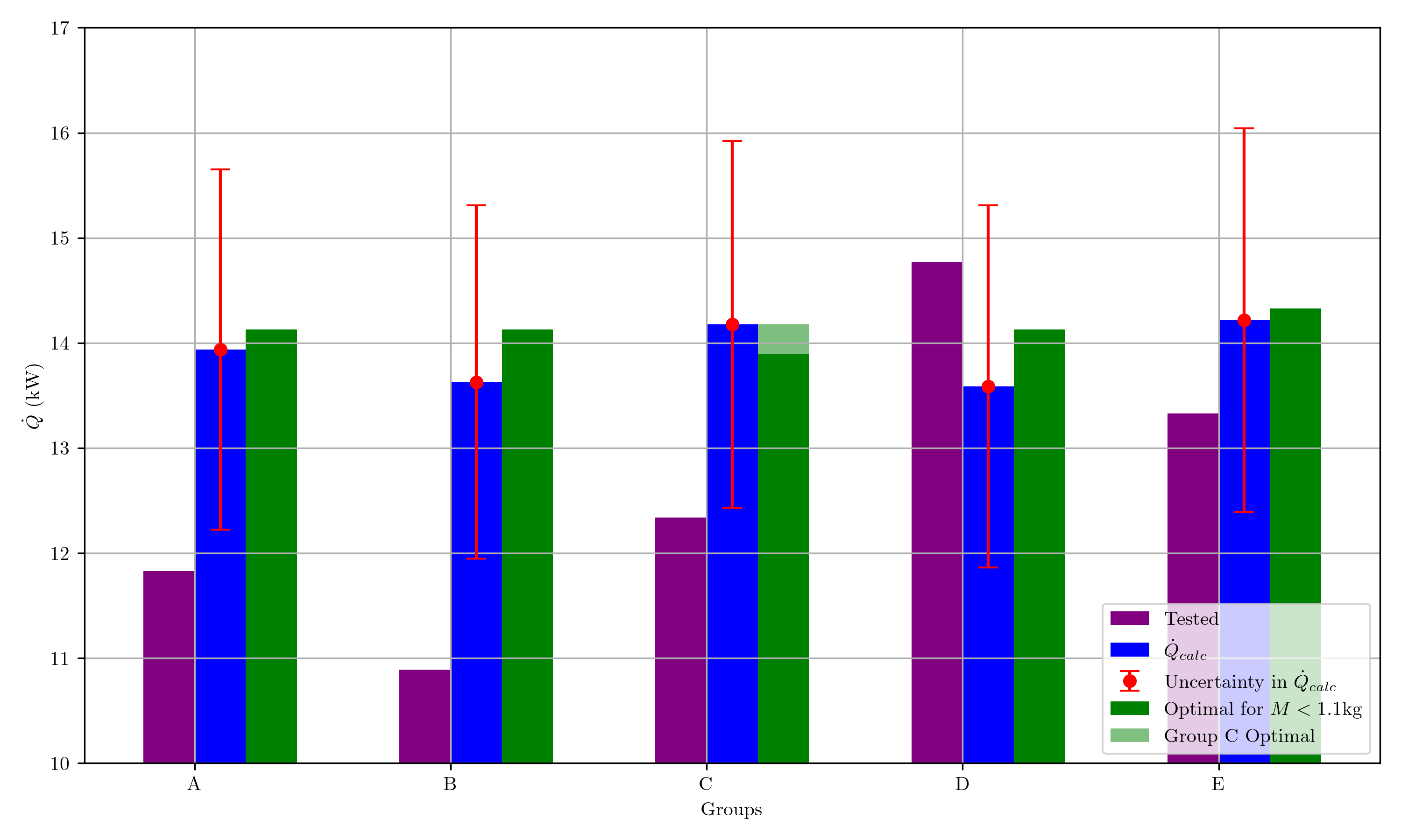 {#fig:Qdot_results width=”60%”}
Figure 3{reference-type=”ref” reference=”fig:Qdot_results”} shows the experimental results for the heat exchanger performance of each group. Group D’s heat exchanger performed the best at 14.77 kW, exceeding our calculated value by 8.7%, but within the uncertainty band of 12.69%. Our group E heat exchanger had the second best performance 9.7% below that of Group D, and 6.2% below our calculated value. The remaining groups ranked C, A and then B at 16.5%, 19.9% and 26.3% below group D, which is the same order predicted by our software. Figure 3{reference-type=”ref” reference=”fig:Qdot_results”} also shows that these last 3 groups are outside of the uncertainty bands with experimental values being -13.0%, -15.1% and -20.1% below the respective calculated values.
Design recommendations
An odd number of hot passes, with more counterflow passes than coflow passes, has a slightly better effectiveness than an even number of hot passes with an equal number of coflow and counterflow. Textbooks state these uncommon designs may result in structural and thermal problems [@HeatTransfer]. However for this application of compact heat exchangers, the lengths and operating temperature gradients are small so thermal expansion is negligible. An additional hot pass comes at a cost of increased pressure drop compared to a smaller number of even hot passes, however the increased effectiveness was found to be worth the tradeoff.
Tube count, position and length are the most important factors in determining the heat exchanger performance. Increasing heat transfer area will generally increase the heat transfer rate and can be done by increasing tube count or length. However this needs to be done carefully as increasing the length increases the hot side pressure drop, increasing tube count reduces hot side pressure drop but increases cold side pressure drop. The software also recommended longer designs with more tubes in later hot passes over shorter designs with an equal number of tubes in each hot pass. This is because increasing the heat transfer area at regions of smaller temperature differences increases the overall heat transfer.
Increasing baffles increases the cold side pressure drop, decreasing the mass flow rate, however, it also increases the shell side Nusselt number, and therefore the overall heat transfer coefficient. For a given design there is a point at which the increased heat transfer coefficient is outweighed by the reduction in mass flow rate. Kerns method seemed to overestimate this optimal number of baffles, selecting designs with $\sim20$ baffles. This makes it difficult to recommend this method for selecting the optimal number of baffles and a more detailed Bell-Delaware method should be considered instead. Our group chose to add a constraint such that the baffle spacing was more than half the shell diameter, however due to thickness and nozzle placement, the actual baffle spacing was reduced.
Conclusion
The development of heat exchanger design software provided valuable insights into heat exchangers. Group D’s heat exchanger showed the best performance, exceeding our calculated value by 8.7%, while our design ranked second, performing 6.2% below expectation. The software correctly predicted the performance order of the remaining groups, although their experimental values fell outside the uncertainty bands. The discrepancies between the calculated and experimental results can be attributed to various factors, such as the limitations of Kern’s method in estimating shell-side pressure drop, unforeseen assembly issues, and leaks in some heat exchangers. Recommendations were made for numerous design configurations and a software tool can be modified to set unique or additional constraints for a variety of applications. Future work is discussed which includes implementing the Bell-Delaware method for more accurate shell-side pressure drop calculations and additional constraints and design considerations.
[1] Holman J. P. Heat Transfer. 10th ed. McGraw-Hill, 2010.
[2] Sadik Kakac, Hongtan Liu, Anchasa Pramuanjaroenkij, Heat Exchangers: Selection, Rating, and Thermal Design, Third Edition CRC Press, 2012.
[3] Endres, SC, Sandrock, C, Focke, WW, A Simplicial Homology Algorithm for Lipschitz Optimisation, Journal of Global Optimization, 2018.
Group Photo

