Computational Fluid Dynamics (CFD)
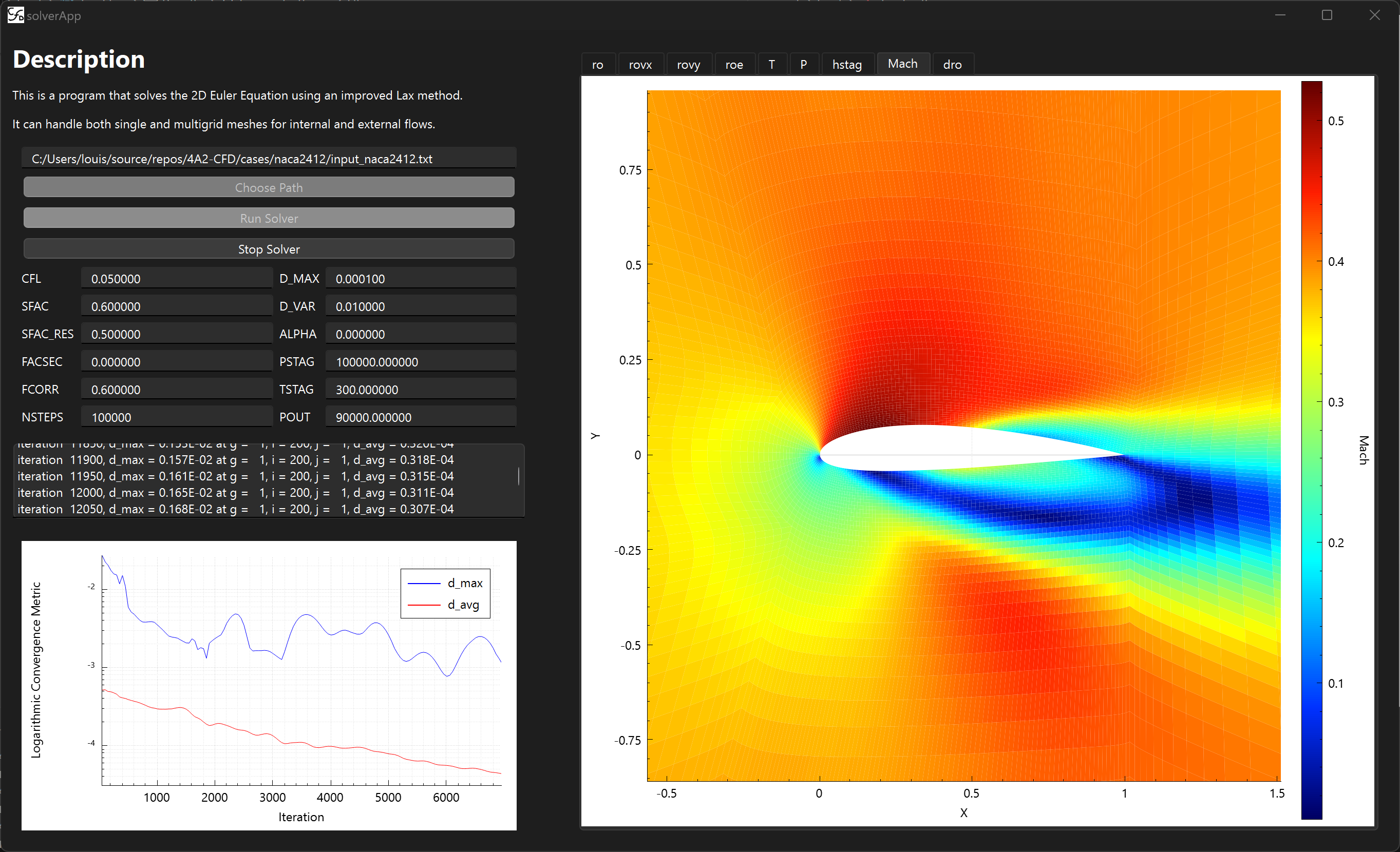
CFD is a powerful tool for solving fluid flow problems. This can be done much faster and at lower cost than experimental methods. This makes it a valuable tool to be used alongside experimental validation
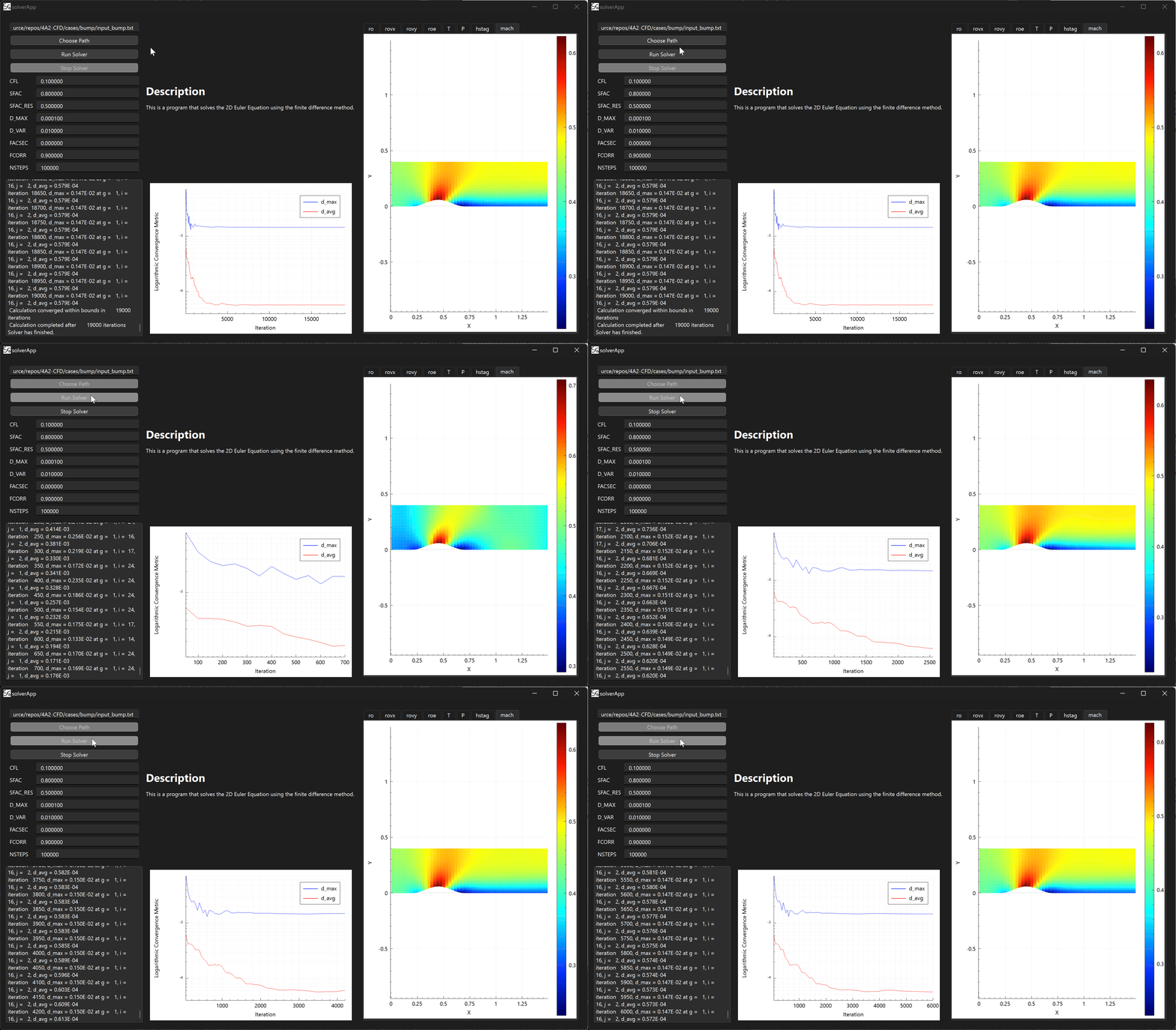
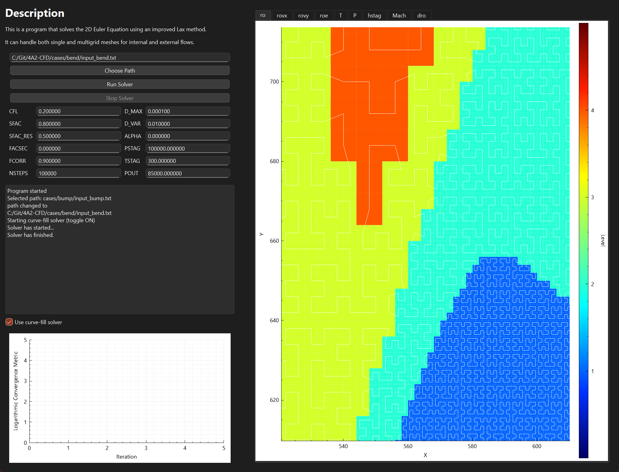
The software is a Qt application that calls fortran routines to solve the Euler equations for a 2D inviscid flow. The user interface is shown above and consists of an input panel and console on the left, a convergence plot in the middle, and various tabs for viewing grid data on the right. The solver routine is ran in a seperate thread to allow the user to interact with graphs and the console while the solver is running. Modifications made to the original code involved binding fortran types to C structs so they could be exchanged between the solver and gui threads to be plotted. This also lays some of the groundwork for future parallelisation of the solver, which may be considered in the improvements if time allows.
Modifications were also made to the convergence criteria to stop the solver when the last 100 calculated d_avg were all within 1% of their mean. This d_avg is the average density residual (change) across all cells in the mesh for a given iteration. This was done to prevent the solver from reaching max iterations when the solution had already converged, making it possible to measure the runtime. However, this could cause the solver to stop prematurely if the convergence was slow, and so the tolerance of 1% may need to be adjusted. The original check if the final residual error is within the bounds specified in the inputs is nested within this check.
This means the solver subroutine will terminate with 4 possible outcomes:
- Converged within boundary specified
- Converged outside boundary specified
- Diverged
- Maximum iterations reached
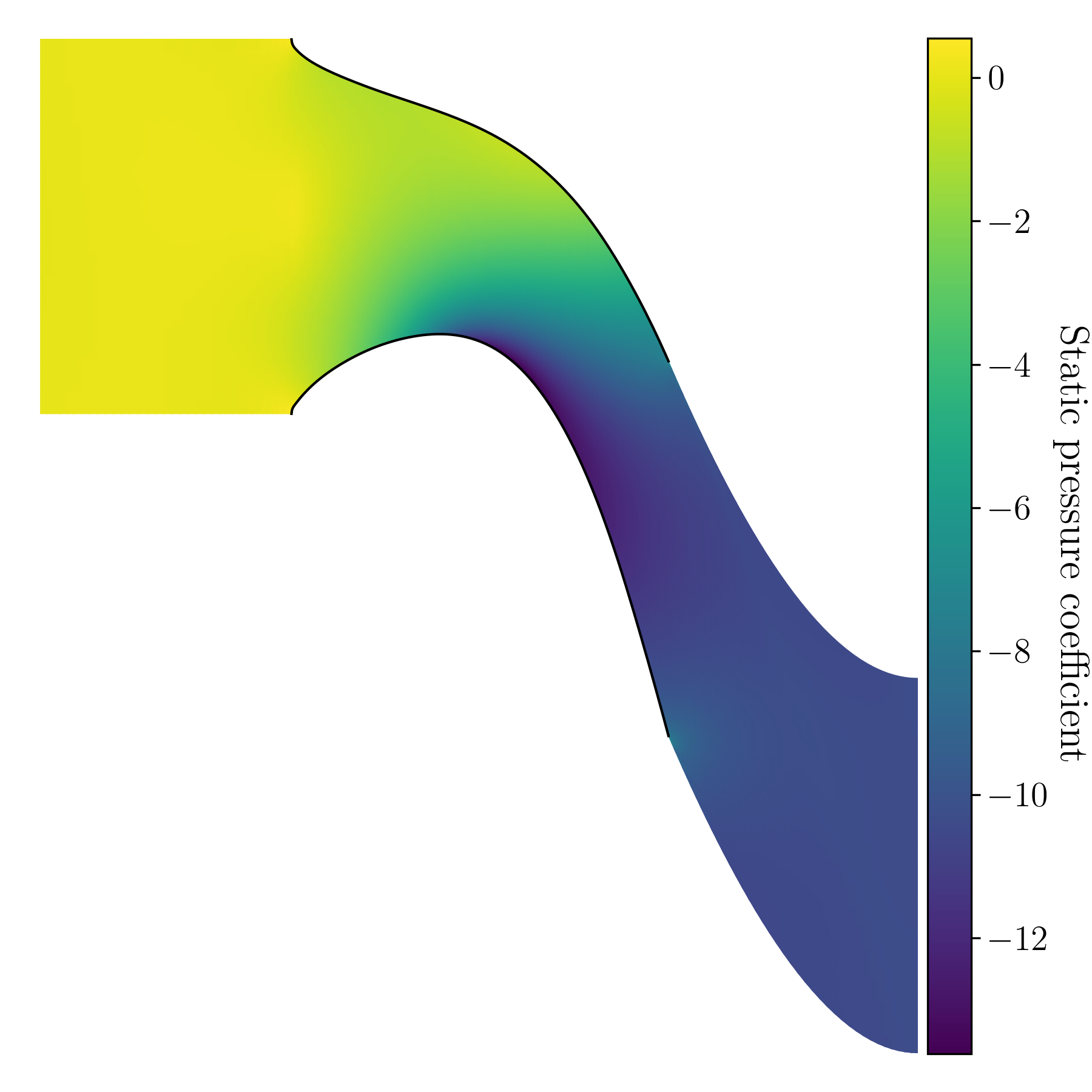
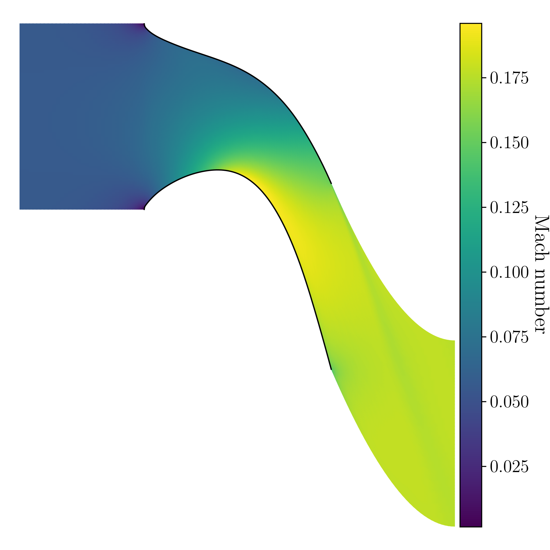
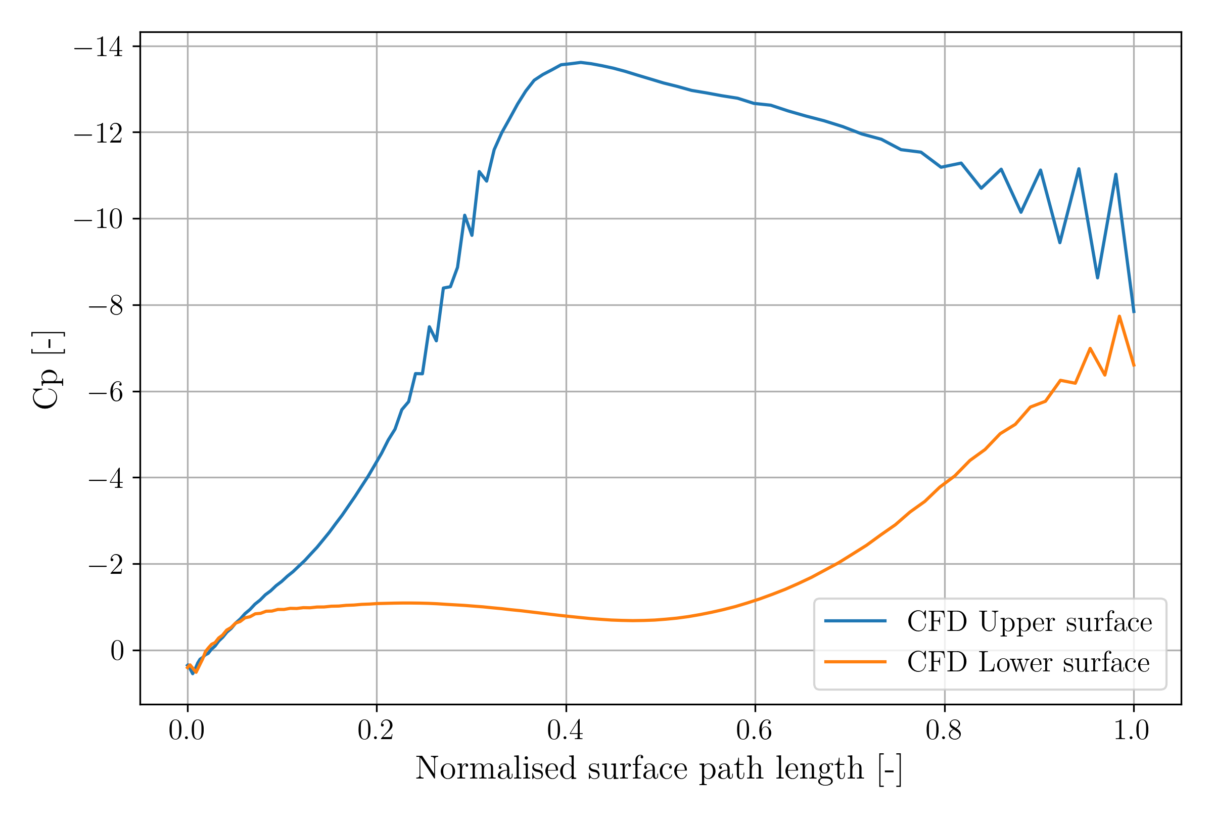
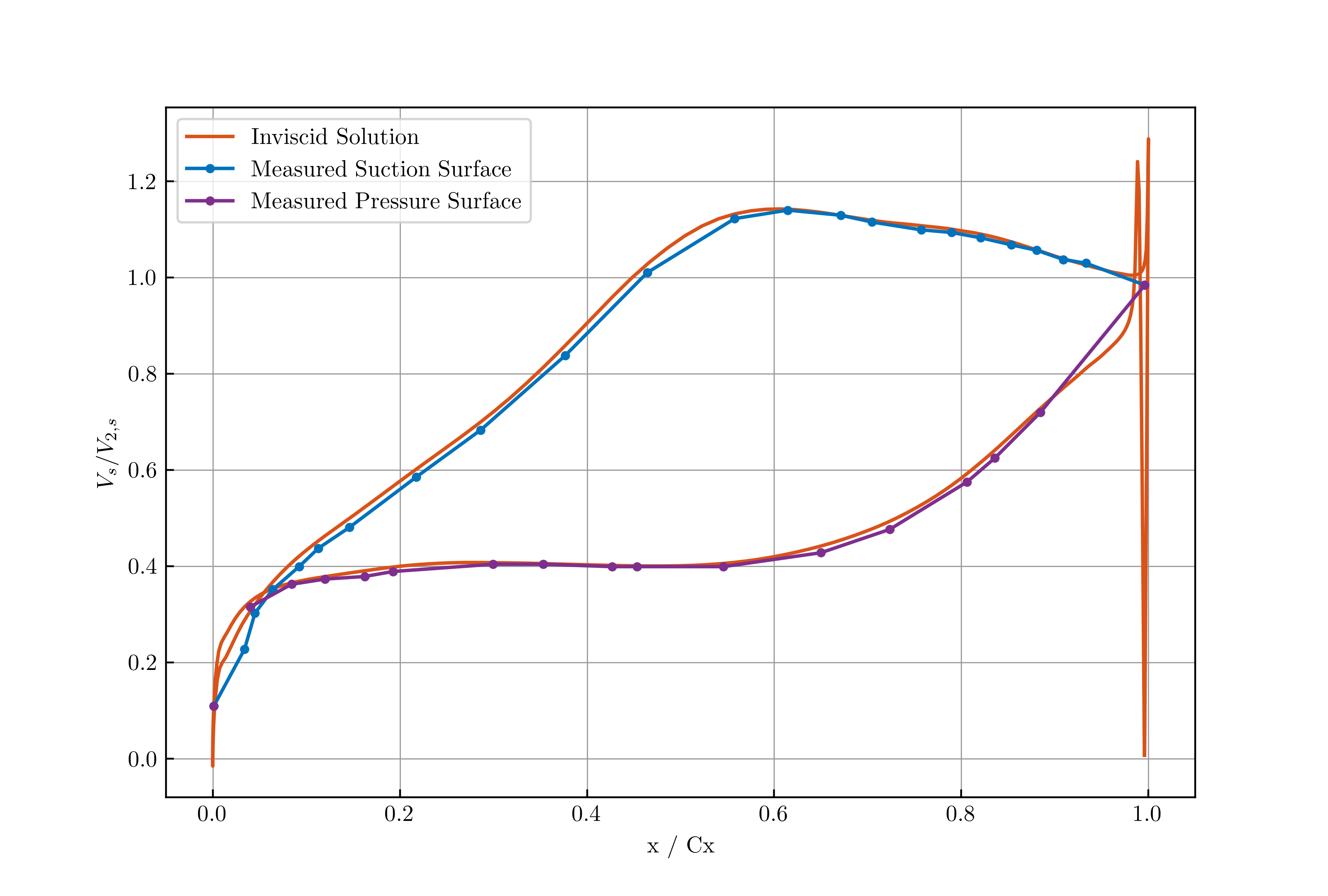
Comparison with real turbine: 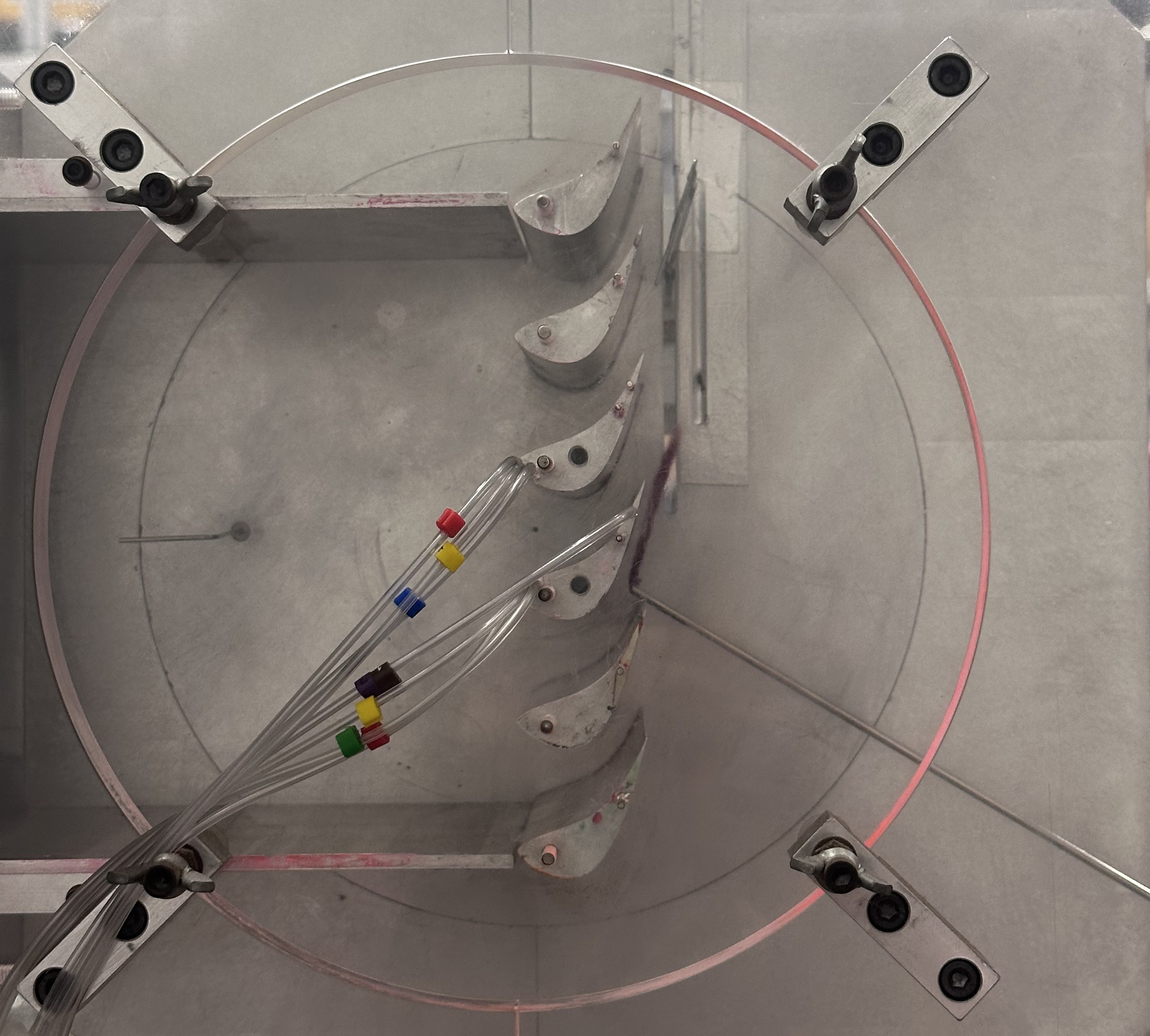
Improvements
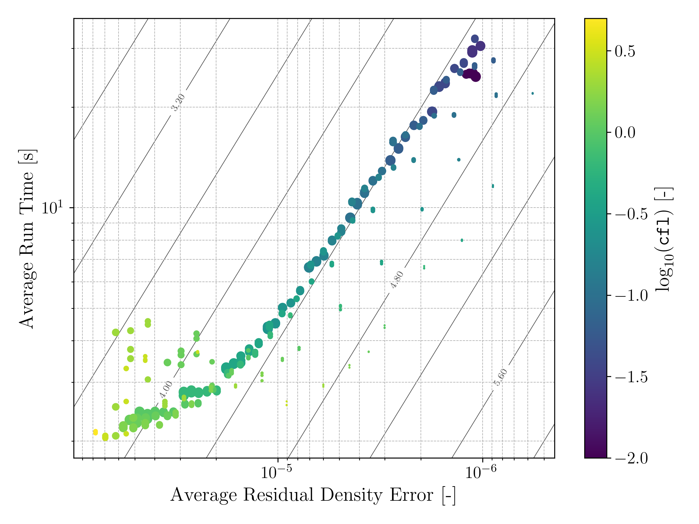
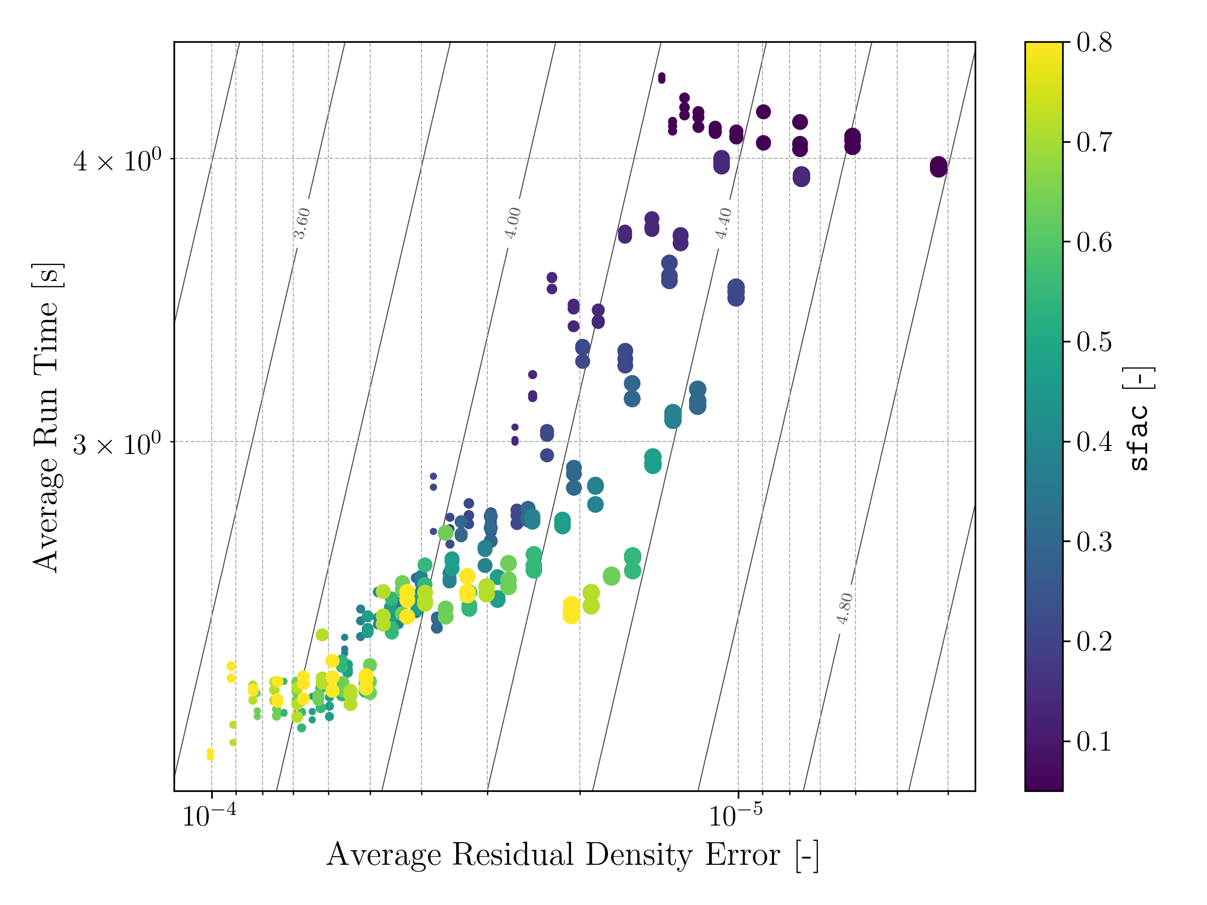
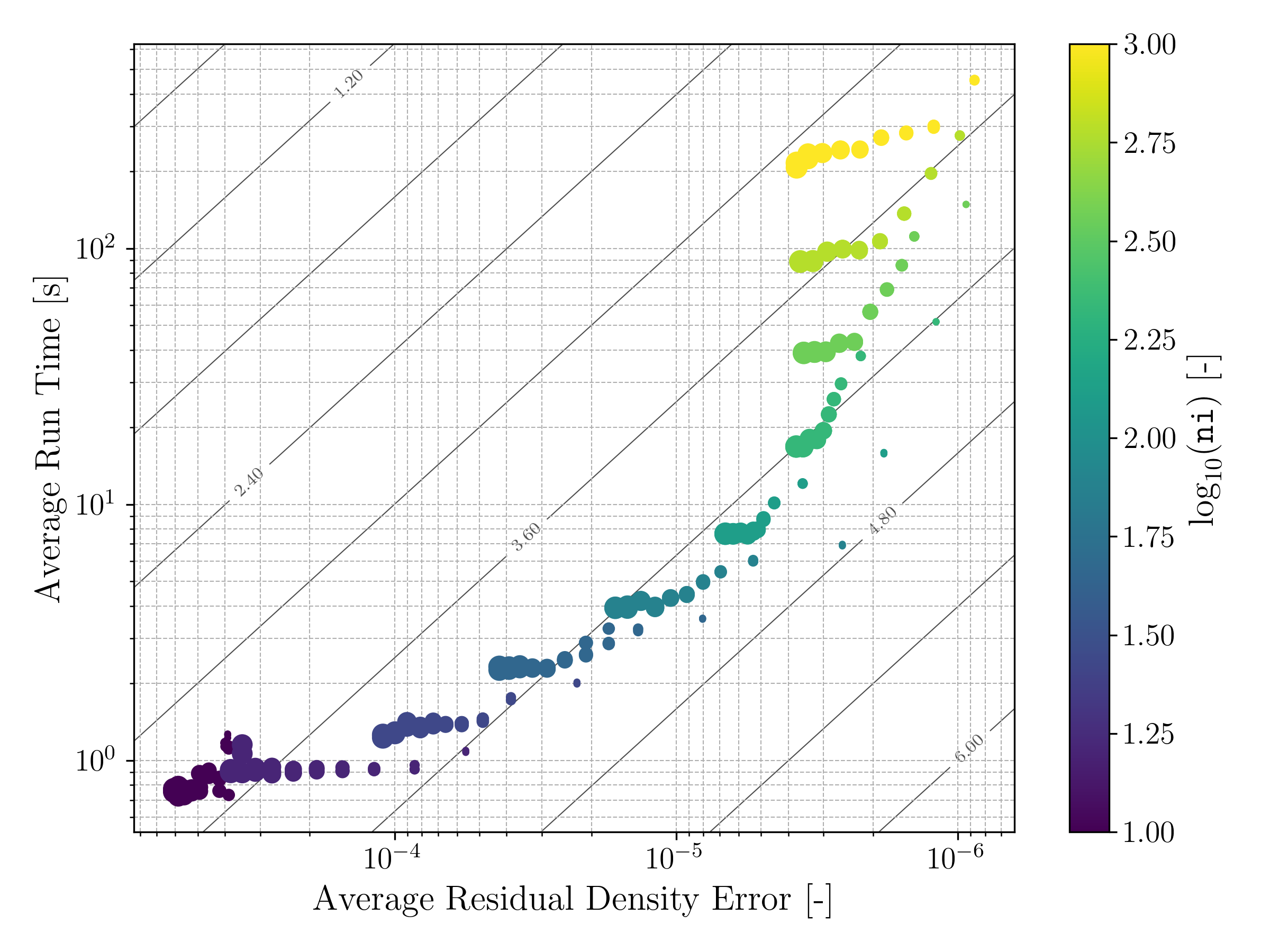
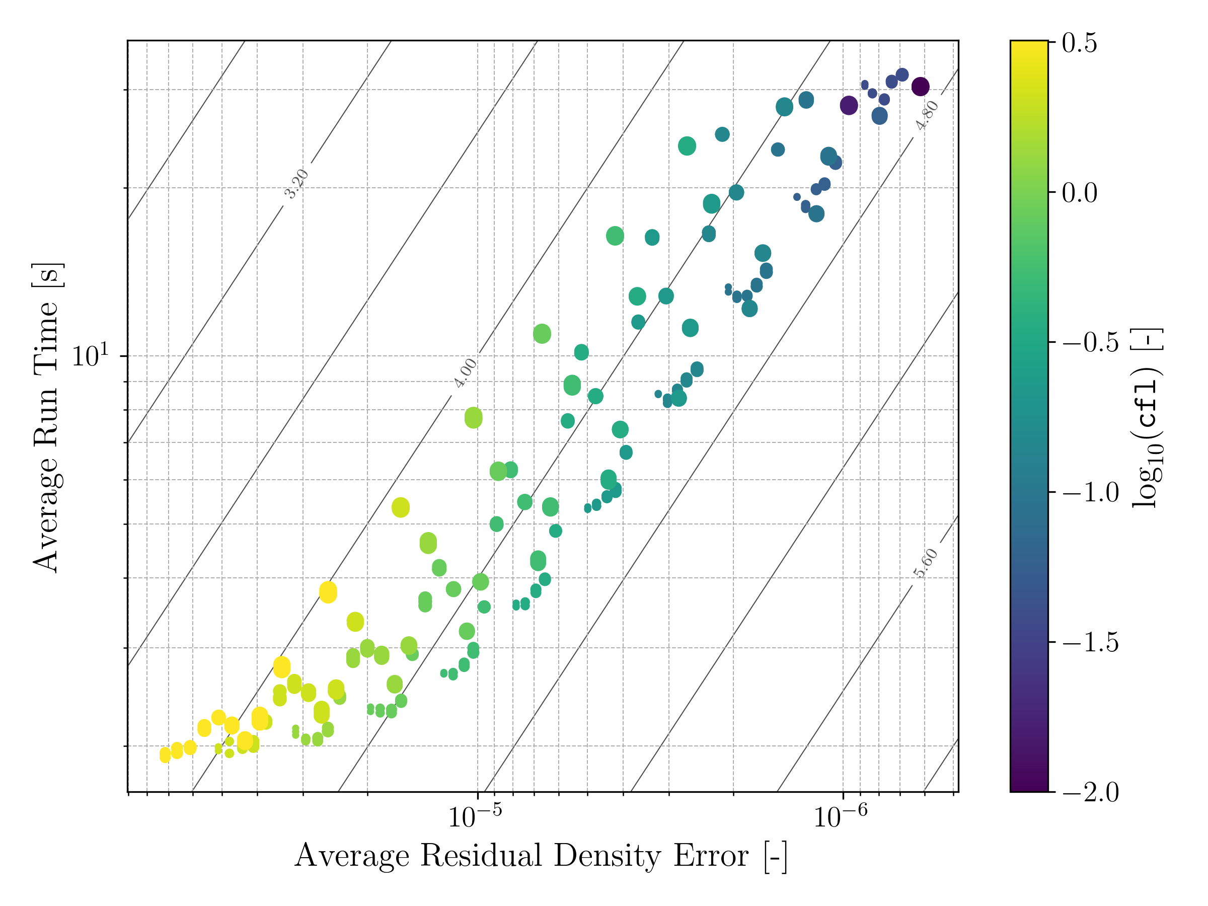
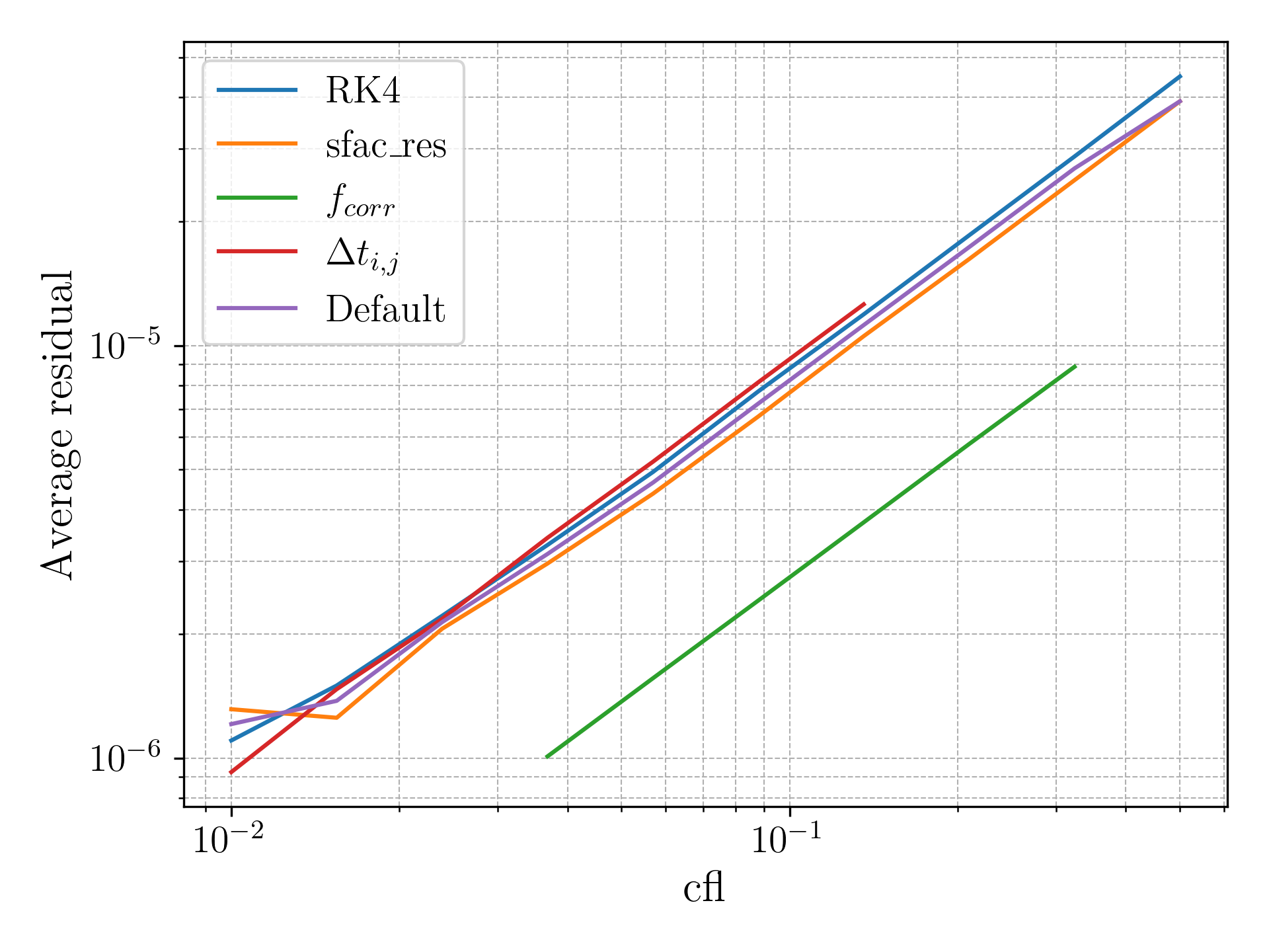
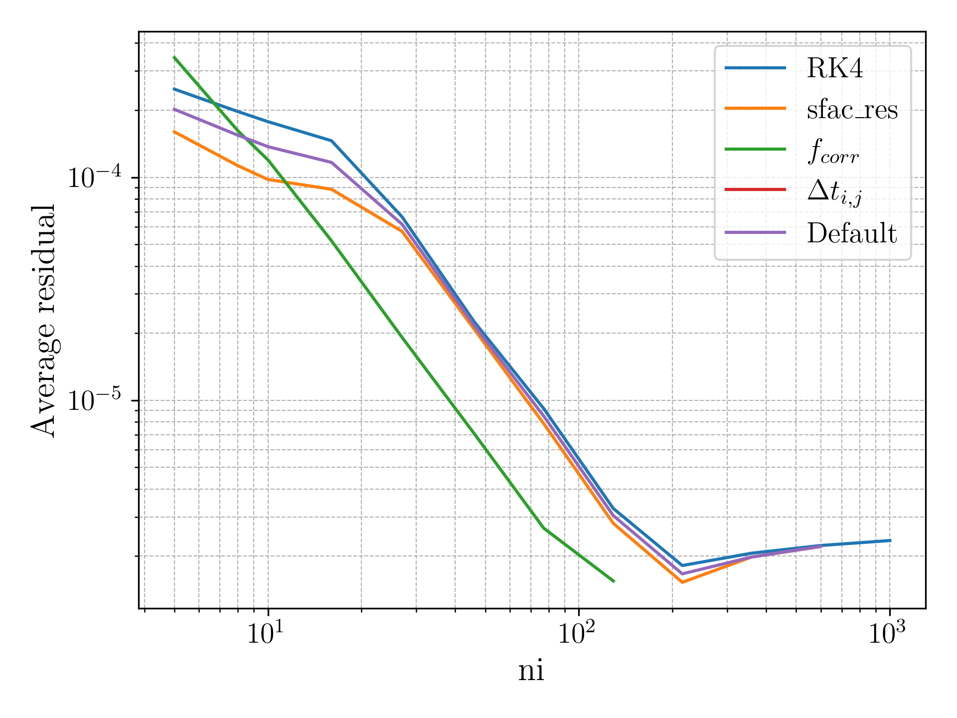
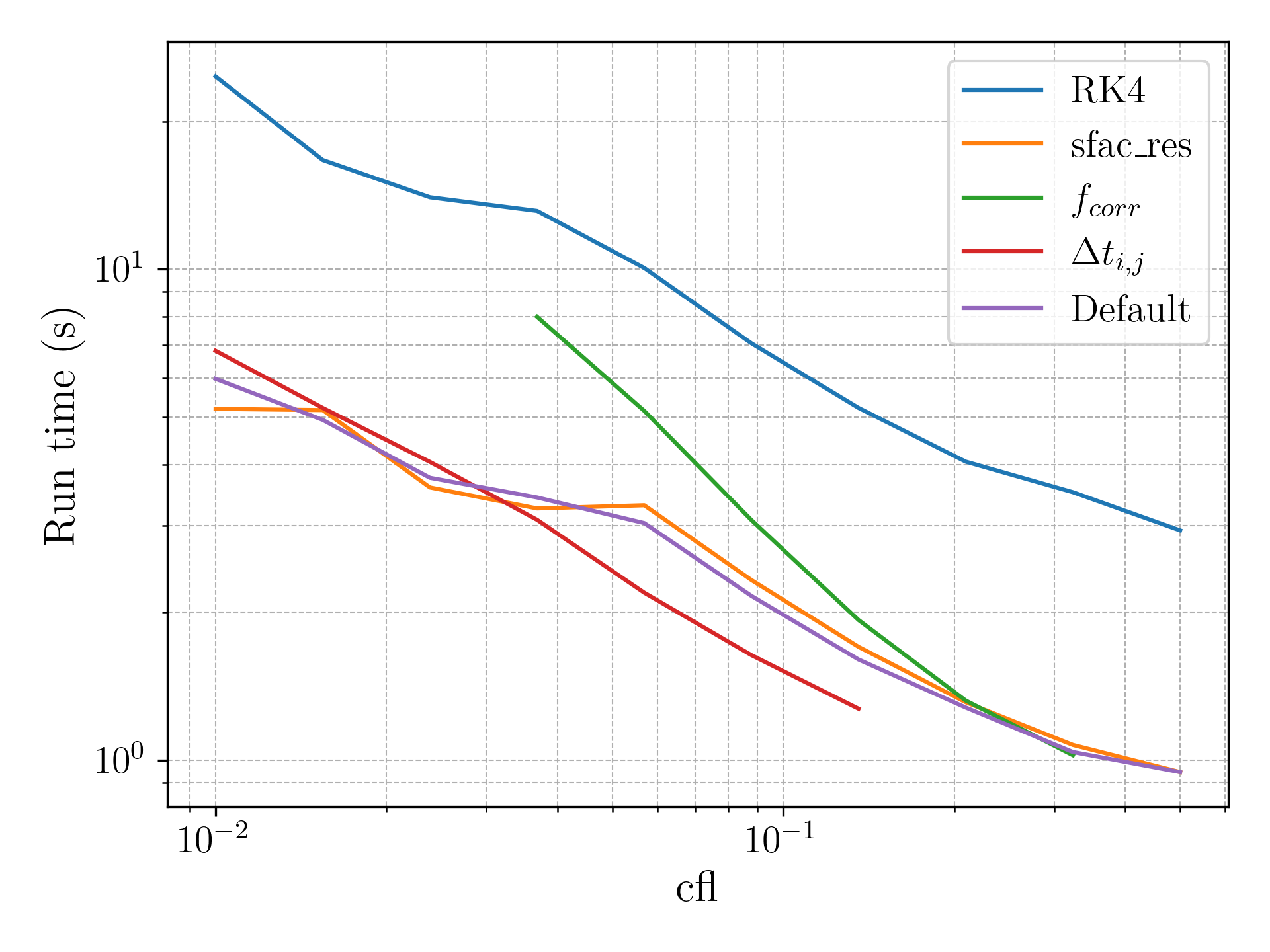
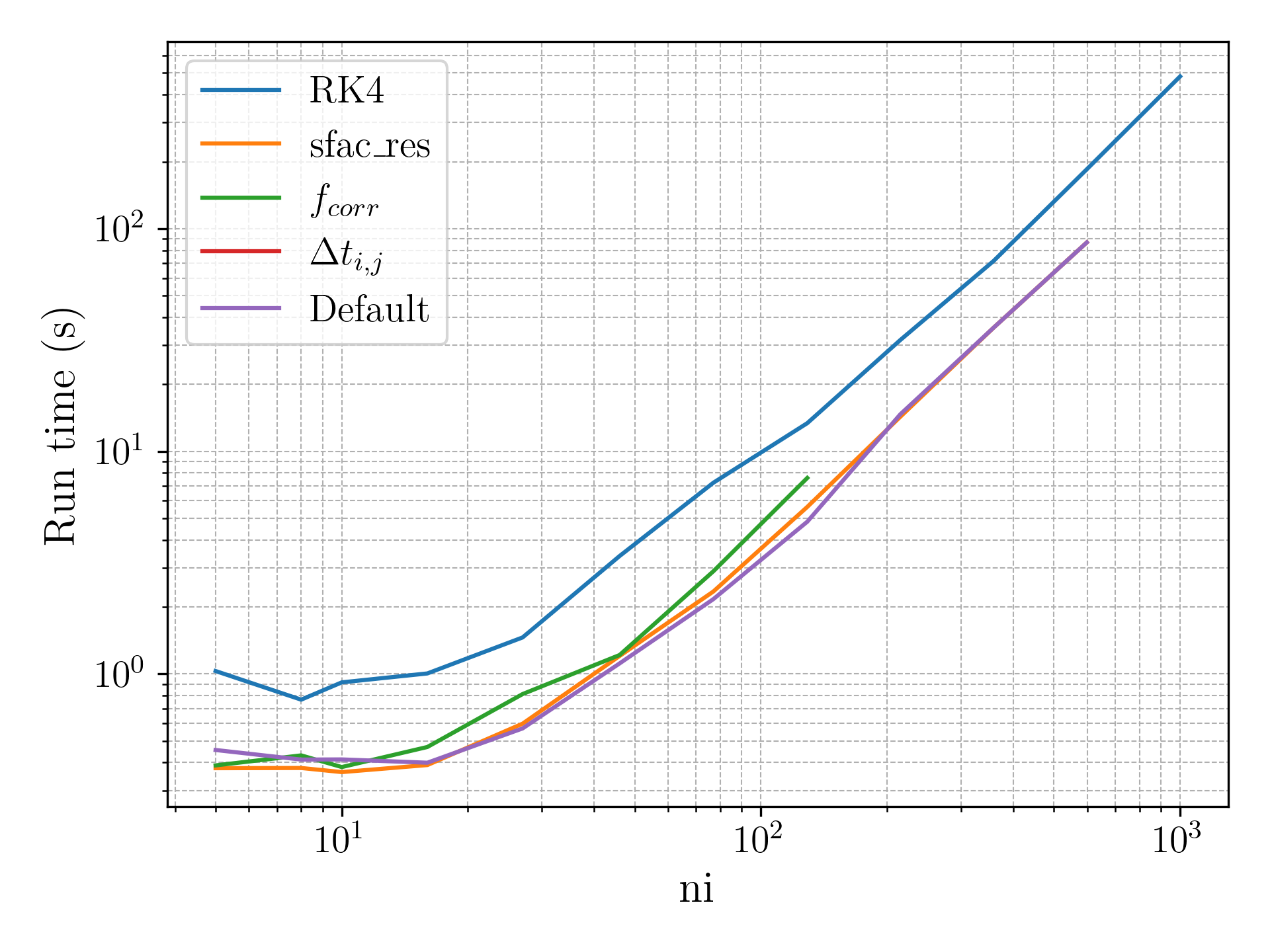
A number of improvements were made and their impact on accuracy and runtime were measured for a range of settings for the generic bump case. These included:
- Runge-Kutta
- Deferred Correction
- Residual Averaging
- Spatially Varying Timestep
The settings at which these improvements were tested over include:
- Courant–Friedrichs–Lewy (CFL) number
- Correction Factor
- Mesh resolution
- Smoothing factor
- Residual smoothing factor
Figure of merit contours can also be seen defined as follows \[\text{FM} = \log_{10} \left( \frac{1}{\texttt{d\_avg} \times T} \right)\]
Future work
Work has begun on a different meshing technique with varying level of detail in a quadtree structure. Space filling curves then structure the data in memory to improve cache performance. This can be seen below where level of detail is based on curvature of the geometry and distance from the cell to the body.
A unsteady flow solver with global maximum timestep update would allow the simulation of transient flows. This would allow for scenarios such as turbine or wind tunnel startup/shutdown, buffeting and dynamic stall.
Include viscous effects to calculate skin friction drag of bodies.
